Using MapLibre and MapTiles in R with mapgl
1 Introduction
Creating interactive maps in R is pretty easy with mapview or leaflet. However, other external libraries such as MapBox or MapLibre have shown a great power for creating web applications. Thanks to Kyle Walker we have access to these powerful libraries using the mapgl package that has been released to CRAN this week. Although the package is in its early stages, we can already do a lot with it.
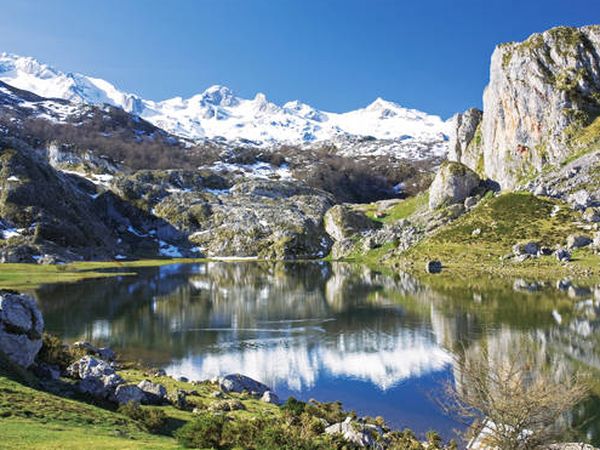
In this tutorial, we will create a map that shows the cycling routes and landmarks in Picos de Europa National Park (Spain):
You will learn:
🗂️ How to unrar files in R
🌐 Download data from Open Street Maps directly into R
🗺️ Use MapLibre and MapTiler in R
🔍 Add vectorial layers to MapLibre and MapTiler (points, lines, and polygons), and customize them adding hover and tooltip effects
📊 Create a legend
Remember that you can find all the code in this repository.
2 Loading packages
We will use the following packages:
archive (Hester and Csárdi 2024): we will use it to unrar files.
fs (Hester et al. 2024): used to create a directory tree.
mapgl (Walker 2024): interface to MapBox GL JS and MapLibre.
mapview (Appelhans et al. 2023): quickly interactive maps for exploration.
osmdata ( et al. 2017): to import Open Street Map features.
tidyverse (tidyverse?): to manipulate data in general.
3 Mapbox, MapLibre and MapTiler
We covered Mapbox in the previous week’s post. Mapbox is a commercial platform that was open source from 2010 to 2020. It’s a JavaScript library for displaying maps using WebGL.
MapLibre was born in December 2020 by a group of contributors who wanted to continue the work of Mapbox as an open source library.
MapTiler is another library that extends the functionality of MapLibre. It has commercial and open source capabilities, and it’s mostly focused on tiles and hosting. We will use it to access the variety of tiles that it has available. Note that you need to create an account in https://www.maptiler.com/.
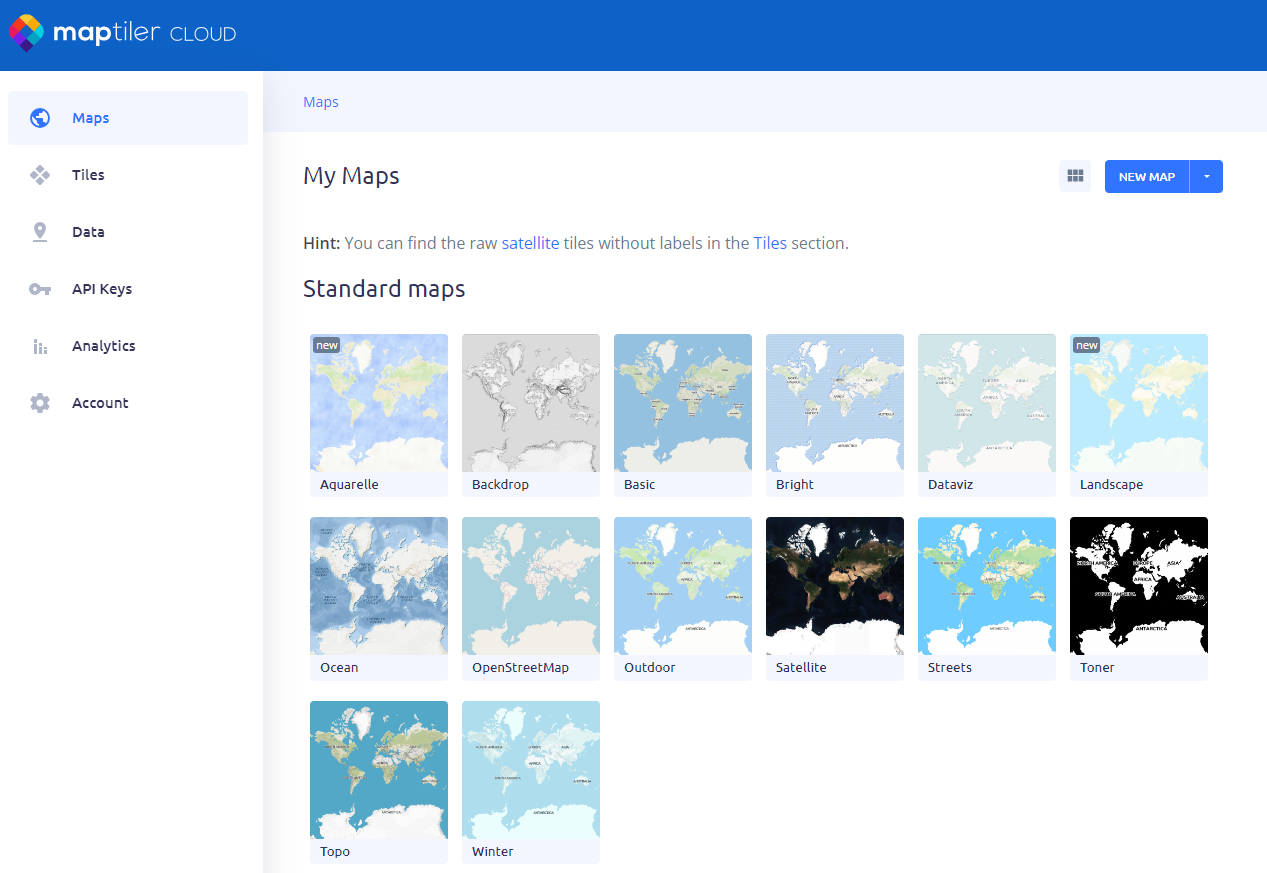
In Figure 2 you can see the tiles that are available to use with the mapgl package. On the left, you can go to API keys to set your environment variable and be able to access your MapTiler cloud. You can follow the next instructions to set the environment variable:

4 Load the data
In this exercise we need to download three sources of data:
Study area (Picos de Europa National Park)
Cycling routes
Landmarks
4.1 Study area
The study area for this exercise is Picos de Europa National Park in Spain. We can download all the data directly from here, and unrar it manually. However, I always prefer to maintain the reproducibility of my scripts as higher as possible maintaining also the source of the data. That’s why we will download the data using R:
## Url to national parks file
url <- "https://www.miteco.gob.es/content/dam/miteco/es/parques-nacionales-oapn/red-parques-nacionales/sig/limites_red_tcm30-452281.rar"

## Define paths for download and unrar
rar_file <- str_glue("{tempdir()}/{basename(url)}")
dest_dir <- str_remove(rar_file, ".rar")

## Download file
download.file(
  url      = url,
  destfile = rar_file,
  mode     = "wb"
)

## unrar file
try(
  archive_extract(rar_file, dest_dir),
  silent = TRUE
)
There, we are defining two paths. One for downloading the rar file, and another for the extracting. We use the archive_extract() function to extract .rar files in R. Note that I need to wrap it within the try() function because it throws an error. However, the function works without problem, as we can wee in the directory tree:
fs::dir_tree(dest_dir)C:\Users\Cidre\AppData\Local\Temp\Rtmp08OmU3/limites_red_tcm30-452281
└── limites_red
├── desc_Red_PN_LIM_Enero2023.rar
├── Limites_PPNN.rar
└── Metadatos_Limites_PN.pdfNow, we need to extract desc_Red_PN_LIM_Enero2023.rar because the spatial data in located inside that folder:
C:\Users\Cidre\AppData\Local\Temp\Rtmp08OmU3/limites_red_tcm30-452281
├── desc_Red_PN_LIM_Enero2023
│   ├── Limites_PPNN.kml
│   ├── Limite_PN_c.cpg
│   ├── Limite_PN_c.dbf
│   ├── Limite_PN_c.prj
│   ├── Limite_PN_c.sbn
│   ├── Limite_PN_c.sbx
│   ├── Limite_PN_c.shp
│   ├── Limite_PN_c.shp.xml
│   ├── Limite_PN_c.shx
│   ├── Limite_PN_p_b.cpg
│   ├── Limite_PN_p_b.dbf
│   ├── Limite_PN_p_b.prj
│   ├── Limite_PN_p_b.sbn
│   ├── Limite_PN_p_b.sbx
│   ├── Limite_PN_p_b.shp
│   ├── Limite_PN_p_b.shp.xml
│   ├── Limite_PN_p_b.shx
│   ├── metadata.xml
│   ├── Metadatos_Limites_PN.pdf
│   └── Modelo_Datos_LIMITES.xlsx
└── limites_red
    ├── desc_Red_PN_LIM_Enero2023.rar
    ├── Limites_PPNN.rar
    └── Metadatos_Limites_PN.pdf
Now we can finally read the data into R using the sf package:
## Read national parks
national_parks_sf <-
  paste0(dest_dir, "/desc_Red_PN_LIM_Enero2023/Limite_PN_p_b.shp") |>
  read_sf()

## Glimpse the data
national_parks_sf |> glimpse()
Rows: 13
Columns: 10
$ Nom_Parque <chr> "20", "06", "24", "03", "13", "01", "02", "08", "04", "07",…
$ Declaracio <chr> "Ley 1/2007, de 2 de marzo", "RD 16/08/1918, declaración de…
$ Reclasific <chr> NA, "Ley 52/1982, de 13 de julio de reclasificación y ampli…
$ Ampliacion <chr> NA, "Ley 52/1982, de 13 de julio de reclasificación y ampli…
$ Fecha_Dec <date> 2007-03-02, 1918-08-16, 2013-07-07, 1973-06-28, 2002-07-01…
$ Sup_proyec <dbl> 18009.968, 15691.174, 33959.877, 3010.614, 8492.487, 53374.…
$ Sist_Coord <chr> "ETRS89-30N", "ETRS89-31N", "ETRS89-30N", "ETRS89-30N", "ET…
$ Modificaci <chr> NA, NA, NA, NA, "Ley 15/2002, de 1 de julio modificada por …
$ d_Nom_Parq <chr> "Parque Nacional de Monfragüe", "Parque Nacional de Ordesa …
$ geometry <MULTIPOLYGON [m]> MULTIPOLYGON (((251826.2 44..., MULTIPOLYGON (…Now we need to filter only one National Park, and transform the data to WGS 84, since it’s needed to retrieve data from Open Street Map (OSM):
picos_europa_sf <- national_parks_sf |>
  filter(
    str_detect(d_Nom_Parq, "Picos de Europa")
  ) |>
  st_transform(4326)
4.2 Cycling routes
Now we need to somehow download the cycling routes into R. We have those features in the OSM dataset that we can access through the osmdata package. We can see all the features available using the next function:
available_features() [1] "4wd_only" "abandoned"
[3] "abutters" "access"
[5] "addr" "addr:city"
[7] "addr:conscriptionnumber" "addr:country"
[9] "addr:county" "addr:district"
[11] "addr:flats" "addr:full"
[13] "addr:hamlet" "addr:housename"
[15] "addr:housenumber" "addr:inclusion"
[17] "addr:interpolation" "addr:place"
[19] "addr:postbox" "addr:postcode"
[21] "addr:province" "addr:state"
[23] "addr:street" "addr:subdistrict"
[25] "addr:suburb" "addr:unit"
[27] "admin_level" "aeroway"
[29] "agricultural" "alcohol"
[31] "alt_name" "amenity"
[33] "area" "atv"
[35] "backward" "barrier"
[37] "basin" "bdouble"
[39] "bicycle" "bicycle_road"
[41] "biergarten" "boat"
[43] "border_type" "boundary"
[45] "brand" "bridge"
[47] "building" "building:architecture"
[49] "building:colour" "building:fireproof"
[51] "building:flats" "building:material"
[53] "building:min_level" "building:part"
[55] "building:soft_storey" "bus_bay"
[57] "busway" "capacity"
[59] "castle_type" "change"
[61] "charge" "clothes"
[63] "construction" "construction#Railways"
[65] "construction_date" "covered"
[67] "craft" "crossing"
[69] "crossing:island" "cuisine"
[71] "cutting" "cycleway"
[73] "cycleway:left" "cycleway:left:oneway"
[75] "cycleway:right" "cycleway:right:oneway"
[77] "denomination" "destination"
[79] "diet:*" "direction"
[81] "dispensing" "disused"
[83] "dog" "drinking_water"
[85] "drinking_water:legal" "drive_in"
[87] "drive_through" "ele"
[89] "electric_bicycle" "electrified"
[91] "embankment" "embedded_rails"
[93] "emergency" "end_date"
[95] "entrance" "est_width"
[97] "fee" "female"
[99] "fire_object:type" "fire_operator"
[101] "fire_rank" "food"
[103] "foot" "footway"
[105] "ford" "forestry"
[107] "forward" "frequency"
[109] "fuel" "gauge"
[111] "golf_cart" "goods"
[113] "hazard" "hazmat"
[115] "healthcare" "healthcare:counselling"
[117] "healthcare:speciality" "height"
[119] "hgv" "highway"
[121] "historic" "horse"
[123] "hot_water" "ice_road"
[125] "incline" "industrial"
[127] "inline_skates" "inscription"
[129] "int_name" "internet_access"
[131] "junction" "kerb"
[133] "landuse" "lane_markings"
[135] "lanes" "lanes:bus"
[137] "lanes:psv" "layer"
[139] "leaf_cycle" "leaf_type"
[141] "leisure" "lhv"
[143] "lit" "loc_name"
[145] "location" "male"
[147] "man_made" "max_age"
[149] "max_level" "maxaxleload"
[151] "maxheight" "maxlength"
[153] "maxspeed" "maxstay"
[155] "maxweight" "maxwidth"
[157] "military" "min_age"
[159] "min_level" "minspeed"
[161] "mofa" "moped"
[163] "motor_vehicle" "motorboat"
[165] "motorcar" "motorcycle"
[167] "motorroad" "mountain_pass"
[169] "mtb:description" "mtb:scale"
[171] "name" "name:left"
[173] "name:right" "name_1"
[175] "name_2" "narrow"
[177] "nat_name" "natural"
[179] "nickname" "noexit"
[181] "non_existent_levels" "nudism"
[183] "office" "official_name"
[185] "old_name" "oneway"
[187] "oneway:bicycle" "openfire"
[189] "opening_hours" "opening_hours:drive_through"
[191] "operator" "orientation"
[193] "oven" "overtaking"
[195] "parking" "parking:condition"
[197] "parking:lane" "passing_places"
[199] "place" "power"
[201] "power_supply" "priority"
[203] "priority_road" "produce"
[205] "proposed" "protected_area"
[207] "psv" "public_transport"
[209] "railway" "railway:preserved"
[211] "railway:track_ref" "recycling_type"
[213] "ref" "ref_name"
[215] "reg_name" "religion"
[217] "religious_level" "rental"
[219] "residential" "roadtrain"
[221] "route" "sac_scale"
[223] "sauna" "service"
[225] "service_times" "shelter_type"
[227] "shop" "short_name"
[229] "shoulder" "shower"
[231] "sidewalk" "site"
[233] "ski" "smoking"
[235] "smoothness" "social_facility"
[237] "sorting_name" "speed_pedelec"
[239] "sport" "start_date"
[241] "step_count" "substation"
[243] "surface" "tactile_paving"
[245] "tank" "tidal"
[247] "toilets" "toilets:wheelchair"
[249] "toll" "topless"
[251] "tourism" "tracks"
[253] "tracktype" "traffic_calming"
[255] "traffic_sign" "trail_visibility"
[257] "trailblazed" "trailblazed:visibility"
[259] "tunnel" "turn"
[261] "type" "unisex"
[263] "usage" "vehicle"
[265] "vending" "voltage"
[267] "water" "wheelchair"
[269] "wholesale" "width"
[271] "winter_road" "wood" We can also see the tags that are available for each of the features:
available_tags("route")# A tibble: 22 × 2
Key Value
<chr> <chr>
1 route bicycle
2 route bus
3 route canoe
4 route detour
5 route ferry
6 route foot
7 route hiking
8 route horse
9 route inline_skates
10 route light_rail
# ℹ 12 more rowsIn this case, we are interested in the feature route and the tag bicycle. To retrieve the data from the API, we need to construct a query defining a bounding box, and the feature we want. After that, we specify the format that we want for the data (sf):
## Cycling routes in the bounding box of the National Park
cycling_routes_osm <- opq(
  bbox = st_bbox(picos_europa_sf)
) |>
  add_osm_feature(
    key   = "route",
    value = "bicycle"
  ) |>
  osmdata_sf()
## Print
cycling_routes_osm
By default, we have a special list with different elements. We are interested in the multilines:
## Extract routes
cycling_routes_sf <- cycling_routes_osm$osm_multilines
## Print
cycling_routes_sf
Simple feature collection with 16 features and 12 fields
Geometry type: MULTILINESTRING
Dimension: XY
Bounding box: xmin: -5.138023 ymin: 43.06694 xmax: -4.613694 ymax: 43.31263
Geodetic CRS: WGS 84
First 10 features:
osm_id name
9509676-backward 9509676 [CIMA LE10] Panderruedas * Caín
9509732-forward 9509732 [CIMA LE10] Panderruedas * Puente Vidosa
9512922-backward 9512922 [CIMA LE15] Pandetrave
9512922-forward 9512922 [CIMA LE15] Pandetrave
9520652-backward 9520652 [CIMA AS02] Amieva
9520652-forward 9520652 [CIMA AS02] Amieva
9521183-backward 9521183 [CIMA AS04] Casielles
9521183-forward 9521183 [CIMA AS04] Casielles
9521324-forward 9521324 [CIMA AS05] Jitu de Escarandi (Collado Barreda)
9530197-forward 9530197 [CIMA AS07] Lagos de Covadonga
role ascent distance mtb:scale:apm network operator
9509676-backward backward 965 18.8 238 ncn CIMA
9509732-forward forward 1180 29.8 179 ncn CIMA
9512922-backward backward 1077 19 274 ncn CIMA
9512922-forward forward 1077 19 274 ncn CIMA
9520652-backward backward 659 7.8 254 ncn CIMA
9520652-forward forward 659 7.8 254 ncn CIMA
9521183-backward backward 467 3.85 198 ncn CIMA
9521183-forward forward 467 3.85 198 ncn CIMA
9521324-forward forward 1090 14.5 285 ncn CIMA
9530197-forward forward 962 14 271 ncn CIMA
ref route source type
9509676-backward CIMA LE10-1 bicycle https://retocima.es route
9509732-forward CIMA LE10-2 bicycle https://retocima.es route
9512922-backward CIMA LE15 bicycle https://retocima.es route
9512922-forward CIMA LE15 bicycle https://retocima.es route
9520652-backward CIMA AS02 bicycle https://retocima.es route
9520652-forward CIMA AS02 bicycle https://retocima.es route
9521183-backward CIMA AS04 bicycle https://retocima.es route
9521183-forward CIMA AS04 bicycle https://retocima.es route
9521324-forward CIMA AS05 bicycle https://retocima.es route
9530197-forward CIMA AS07 bicycle https://retocima.es route
geometry
9509676-backward MULTILINESTRING ((-4.903486...
9509732-forward MULTILINESTRING ((-5.09084 ...
9512922-backward MULTILINESTRING ((-4.903486...
9512922-forward MULTILINESTRING ((-4.916104...
9520652-backward MULTILINESTRING ((-5.124228...
9520652-forward MULTILINESTRING ((-5.137599...
9521183-backward MULTILINESTRING ((-5.086836...
9521183-forward MULTILINESTRING ((-5.077389...
9521324-forward MULTILINESTRING ((-4.830428...
9530197-forward MULTILINESTRING ((-5.059753...We can see that some names are repeated because some routes have forward and backward path. We will dissolve those elements into one depending on the name attribute:
## Dissolve by name
cycling_routes_united_sf <- cycling_routes_sf |>
  group_by(name) |>
  summarise(
    geometry = st_union(geometry)
  )
## Print
cycling_routes_united_sf
Simple feature collection with 11 features and 1 field
Geometry type: GEOMETRY
Dimension: XY
Bounding box: xmin: -5.138023 ymin: 43.06694 xmax: -4.613694 ymax: 43.31263
Geodetic CRS: WGS 84
# A tibble: 11 × 2
name geometry
<chr> <GEOMETRY [°]>
1 [CIMA AS02] Amieva MULTILINESTRING ((-5.078675 …
2 [CIMA AS04] Casielles MULTILINESTRING ((-5.090698 …
3 [CIMA AS05] Jitu de Escarandi (Collado Barreda) LINESTRING (-4.830428 43.258…
4 [CIMA AS07] Lagos de Covadonga LINESTRING (-5.059753 43.312…
5 [CIMA AS18] Collada Llómena * Puente Vidosa MULTILINESTRING ((-5.138023 …
6 [CIMA AS37] Collada Trespandiu LINESTRING (-4.753377 43.296…
7 [CIMA CA03] San Glorio - Collada de Llesba LINESTRING (-4.620437 43.155…
8 [CIMA CA13] La Hoja - Salto de la Cabra MULTILINESTRING ((-4.662783 …
9 [CIMA LE10] Panderruedas * Caín LINESTRING (-5.013508 43.099…
10 [CIMA LE10] Panderruedas * Puente Vidosa LINESTRING (-5.09084 43.2095…
11 [CIMA LE15] Pandetrave MULTILINESTRING ((-4.916104 …So now we can see that we have a total of 11 different paths. We can calculate the length of each route, and create some labels using HTML tags for better display on the map:
## Calculate path length, and create labels for the map
cycling_routes_united_sf <- cycling_routes_united_sf |>
  mutate(
    length = st_length(cycling_routes_united_sf) |> units::set_units(km)
  ) |>
  mutate(
    label = str_glue("{name} <br> <b>{round(length, 2)} km</b>")
  )
4.3 Landmarks
We will retrieve the landmarks labelled as viewpoint or attraction. The feature that we are interested in is the tourism:
## OSM tags for tourism
available_tags("tourism") |> pull(Value)
[1] "alpine_hut" "apartment" "aquarium" "artwork"
[5] "attraction" "camp_pitch" "camp_site" "caravan_site"
[9] "chalet" "gallery" "guest_house" "hostel"
[13] "hotel" "information" "motel" "museum"
[17] "picnic_site" "theme_park" "viewpoint" "wilderness_hut"
[21] "yes" "zoo" As before, we need to build an OSM query and retrieve the data:
## Get the viewpoints and attractions
landmarks_osm <- opq(
  bbox = st_bbox(picos_europa_sf)
) |>
  add_osm_feature(
    key   = "tourism",
    value = c("viewpoint", "attraction")
  ) |>
  osmdata_sf()
## Print the points
landmarks_osm$osm_points
Simple feature collection with 73 features and 26 fields
Geometry type: POINT
Dimension: XY
Bounding box: xmin: -5.109304 ymin: 43.07675 xmax: -4.619224 ymax: 43.31525
Geodetic CRS: WGS 84
First 10 features:
osm_id name addr:street
248862660 248862660 Mirador de los Canónigos <NA>
282969055 282969055 Mirador del Picu Urriellu <NA>
434307223 434307223 <NA> <NA>
491445504 491445504 Mirador del Corzo <NA>
637622154 637622154 Puerto de Panderrueda <NA>
672438605 672438605 Mirador del Tombo <NA>
687454795 687454795 Mirador de Piedrashitas <NA>
697949257 697949257 Mirador de Vistalegre <NA>
829952039 829952039 Mirador del Príncipe <NA>
1101023501 1101023501 Cueva de Cuadonga <NA>
alt_name direction ele highway historic key
248862660 <NA> <NA> <NA> <NA> <NA> <NA>
282969055 Mirador del Pozu de la Oración <NA> <NA> <NA> <NA> <NA>
434307223 <NA> <NA> <NA> <NA> <NA> <NA>
491445504 <NA> <NA> <NA> <NA> <NA> <NA>
637622154 <NA> <NA> <NA> <NA> <NA> <NA>
672438605 <NA> <NA> <NA> <NA> <NA> <NA>
687454795 <NA> <NA> <NA> <NA> <NA> <NA>
697949257 <NA> <NA> <NA> <NA> <NA> <NA>
829952039 <NA> <NA> <NA> <NA> <NA> <NA>
1101023501 <NA> <NA> <NA> <NA> <NA> <NA>
mapillary name:de name:en name:es natural not:name note
248862660 <NA> <NA> <NA> <NA> <NA> <NA> <NA>
282969055 <NA> <NA> <NA> <NA> <NA> <NA> <NA>
434307223 <NA> <NA> <NA> <NA> <NA> <NA> <NA>
491445504 <NA> <NA> <NA> <NA> <NA> <NA> <NA>
637622154 <NA> <NA> <NA> <NA> <NA> <NA> <NA>
672438605 <NA> <NA> <NA> <NA> <NA> <NA> <NA>
687454795 <NA> <NA> <NA> <NA> <NA> <NA> <NA>
697949257 <NA> <NA> <NA> <NA> <NA> <NA> <NA>
829952039 <NA> <NA> <NA> <NA> <NA> <NA> <NA>
1101023501 <NA> <NA> <NA> <NA> <NA> <NA> <NA>
opening_hours ruins source source:date start_date survey:date
248862660 <NA> <NA> <NA> <NA> <NA> <NA>
282969055 <NA> <NA> <NA> <NA> <NA> <NA>
434307223 <NA> <NA> <NA> <NA> <NA> <NA>
491445504 <NA> <NA> <NA> <NA> <NA> <NA>
637622154 <NA> <NA> <NA> <NA> <NA> <NA>
672438605 <NA> <NA> <NA> <NA> <NA> <NA>
687454795 <NA> <NA> ITACyL 20100407 <NA> <NA>
697949257 <NA> <NA> <NA> <NA> <NA> <NA>
829952039 <NA> <NA> <NA> <NA> <NA> <NA>
1101023501 <NA> <NA> PNOA <NA> <NA> <NA>
tourism wheelchair wikidata wikipedia
248862660 viewpoint <NA> <NA> <NA>
282969055 viewpoint <NA> <NA> <NA>
434307223 viewpoint <NA> <NA> <NA>
491445504 viewpoint <NA> <NA> <NA>
637622154 viewpoint <NA> <NA> <NA>
672438605 viewpoint <NA> Q17622552 es:Mirador del Tombo
687454795 viewpoint <NA> <NA> <NA>
697949257 viewpoint <NA> <NA> <NA>
829952039 viewpoint <NA> <NA> <NA>
1101023501 viewpoint <NA> <NA> <NA>
geometry
248862660 POINT (-5.043759 43.30529)
282969055 POINT (-4.839009 43.31155)
434307223 POINT (-4.691411 43.10503)
491445504 POINT (-4.733009 43.07677)
637622154 POINT (-4.981941 43.12496)
672438605 POINT (-4.90376 43.171)
687454795 POINT (-4.980282 43.12907)
697949257 POINT (-5.051131 43.14847)
829952039 POINT (-4.983474 43.27841)
1101023501 POINT (-5.054411 43.30732)We are interested in the points. We will classify them as Viewpoint or Other. To do so, we need first to populate all the NA values on the name column as Unidenfied. After that, we can classify them in a new column called type:
Simple feature collection with 73 features and 2 fields
Geometry type: POINT
Dimension:     XY
Bounding box:  xmin: -5.109304 ymin: 43.07675 xmax: -4.619224 ymax: 43.31525
Geodetic CRS:  WGS 84
First 10 features:
                                name      type                   geometry
248862660   Mirador de los Canónigos Viewpoint POINT (-5.043759 43.30529)
282969055  Mirador del Picu Urriellu Viewpoint POINT (-4.839009 43.31155)
434307223               Unidentified     Other POINT (-4.691411 43.10503)
491445504          Mirador del Corzo Viewpoint POINT (-4.733009 43.07677)
637622154      Puerto de Panderrueda     Other POINT (-4.981941 43.12496)
672438605          Mirador del Tombo Viewpoint    POINT (-4.90376 43.171)
687454795    Mirador de Piedrashitas Viewpoint POINT (-4.980282 43.12907)
697949257      Mirador de Vistalegre Viewpoint POINT (-5.051131 43.14847)
829952039       Mirador del Príncipe Viewpoint POINT (-4.983474 43.27841)
1101023501         Cueva de Cuadonga     Other POINT (-5.054411 43.30732)
5 Map
Finally, we can create the final map using MapLibre and MapTiler. Remember that this will only work if you followed the instructions of Figure 3. We have vectorial data representing the three main geometry types:
Study area: represented by a polygon. It will be mapped using
add_fill_layer().Cycling routes: represented by lines. It will be mapped using
add_line_layer().Landmarks: represented by points. It will be mapped using
add_circle_layer().
All of these functions have two mandatory arguments:
id: an unique identifier for the layer
source: the data source. In this case, an
sfobject.
There are other optional arguments that are specific to the geometry type. First, we will create a base map using the satellite tile from MapTiler, fit the bounds to the national park with an animation, and adding some navigation and fullscreen control widgets:
map <- maplibre(
  style  = maptiler_style("satellite"),
)  |>
  fit_bounds(
    picos_europa_sf,
    animate = TRUE
  ) |>
  add_navigation_control() |>
  add_fullscreen_control()
Next, we can add the polygon layer with transparent fill color, and red outline. Note that the current version of {mapl} doesn’t support outline width.
map <- map |>
  add_fill_layer(
    id                 = "picos_europa",
    source             = picos_europa_sf,
    fill_color         = "transparent",
    fill_opacity       = 1,
    fill_outline_color = "red"
  )
Now we will add the cycling routes on top of the previous layer. We add the tooltip argument where we can specify a column name to show when we hover the geometries. The argument hover_options takes a list where we can specify specific options to the state of hover:
map <- map |>
  add_line_layer(
    id            = "routes",
    source        = cycling_routes_united_sf,
    line_color    = "wheat",
    line_width    = 2,
    tooltip       = "label",
    hover_options = list(
      line_color = "red",
      line_width = 5
    )
  )
Finally, we can add the landmarks with a legend based on the type column. In this case, for the circle_color we use a match_expr() to specify the column, the unique values of the column, and a vector of stops (colors).
We can add a categorical legend specifying the values and colors again. Note that the legend is independent from the data, so we have a lot of flexibility to create it.
## Colours for points
point_col <- c("lightcoral", "lavender")

## Map
map <- map |>
  add_circle_layer(
      id                    = "landmarks",
      source                = landmarks_sf,
      popup                 = "name",
      circle_opacity        = 1,
      circle_radius         = 6,
      circle_stroke_color   = "black",
      circle_stroke_opacity = 1,
      circle_stroke_width   = 1,
      circle_color          = match_expr(
        column = "type",
        values = landmarks_sf$type |> unique(),
        stops  = point_col
      ),
    ) |>
    add_categorical_legend(
      legend_title     = "Landmark",
      values           = landmarks_sf$type |> unique(),
      colors           = point_col,
      unique_id        = "landmark_legend",
      circular_patches = TRUE
    )
6 Conclusions
mapgl is an awesome package that allows us to access the Mapbox and MapLibre libraries. This package has been released to CRAN very recently, and although it’s features are already awesome, there are some features that haven’t been added yet. For instance, if you try to add another independent legend, it will overwrite the previous one. We also saw that the polygon’s outline width cannot be adjusted. However, the package it’s in its very early stages and as you could saw in this tutorial you can map all the main vectorial geometries using mapgl. This package is a great achievement for the R community, and you can support the project of Kyle Walker in the GitHub repository.