library(pacman)

p_load(
  ## Core
  tidyverse,

  ## Donwload data
  httr, R.utils,

  ## Spatial data
  sf, stars, terra,

  ## Visualization
  rayshader, colorspace, MetBrewer
)1 Introduction
In this post, we will create an amazing spikes population map for the country of Norway using the awesome {rayshader} R package.
I will use data from the Kontur database, which has a population density dataset where the world population is represented by H3 hexagons with a spatial resolution of 400 meters.
2 Loading packages
If you followed me in other posts or did any of my courses, you will notice that I always use the {pacman} package to load the rest of the packages. This is because the p_load function will install any missing packages, and then load them into our R session.
3 Load the data
The data can be directly downloaded from the Kontur website, or we can also copy the url for the country and download it into R directly.
First I create a function that will download the data using httr::GET(), then it will unzip the gz file with R.utils::gunzip(), and finally it will return the file path without the gz extension.
get_data_httr <- function(url, file_name) {
  ## Get url
  httr::GET(
    url,
    write_disk(file_name)
  )
  ## Unzip the gz file
  R.utils::gunzip(file_name, remove = TRUE)
  ## Get the file path
  gsub(".gz", "", file_name)
}
Then, we apply the function by providing the url to the compressed file, and also the file name with the gz extension:
## Url
url <- "https://geodata-eu-central-1-kontur-public.s3.amazonaws.com/kontur_datasets/kontur_population_NO_20231101.gpkg.gz"
## File name
file_name <- "norway-population.gpkg.gz"

## Get file path
file_path <- get_data_httr(url, file_name)
Once we downloaded the data, we can read it into R and project it to the Lambert Azimuthal Equal-Area (LAEA) projection:
population_sf <-
  read_sf(file_path) %>%
  st_transform("EPSG:3035")

population_sf
Simple feature collection with 186254 features and 2 fields
Geometry type: POLYGON
Dimension: XY
Bounding box: xmin: 3629718 ymin: 3876026 xmax: 5132823 ymax: 6391949
Projected CRS: ETRS89-extended / LAEA Europe
# A tibble: 186,254 × 3
h3 population geom
* <chr> <dbl> <POLYGON [m]>
1 8809abd9b5fffff 2 ((4045387 4292797, 4044957 4292776, 4044823 42923…
2 8809abd9a7fffff 1 ((4044985 4291569, 4044555 4291547, 4044421 42911…
3 8809abcf67fffff 66 ((4054799 4300908, 4054370 4300887, 4054237 43004…
4 8809abcf63fffff 1 ((4054637 4301704, 4054208 4301684, 4054075 43012…
5 8809abcf2dfffff 2 ((4055524 4300541, 4055095 4300520, 4054961 43001…
6 8809abcf2bfffff 6 ((4055924 4301767, 4055495 4301746, 4055362 43013…
7 8809abcf29fffff 6 ((4055362 4301337, 4054933 4301317, 4054799 43009…
8 8809abcf27fffff 5 ((4056811 4300603, 4056382 4300583, 4056248 43001…
9 8809abcf25fffff 2 ((4056248 4300174, 4055819 4300153, 4055686 42997…
10 8809abcf21fffff 7 ((4056086 4300970, 4055657 4300950, 4055524 43005…
# ℹ 186,244 more rowsThe data contains the h3 column which is the ID of the h3 hexagon, and the total population within the hexagon.
[1] TRUE[1] FALSE4 Prepare the data
Once we have the population file loaded into R, we need to convert it into a raster. This is because when working with {rayshader} we need to work with a matrix, and in essence, a raster is a matrix of values.
Therefore, to create the hexagons into a raster, first we need to know the dimensions that we want for our raster. The next function will do the work. First, we get the height and width of the bounding box of our population data. Then we create the ratio variables storing the highest one as 1, and the lowest one as the ratio with the highest:
# Create function to get width and height
get_raster_size <- function(bbox) {
  ## Get height and width in CRS units
  height <- as.vector(bbox[4] - bbox[2])
  width  <- as.vector(bbox[3] - bbox[1])
  ## Get the ratio between height and width
  if (height > width) {
    height_ratio <- 1
    width_ratio <- width / height
  } else {
    width_ratio <- 1
    height_ratio <- height / width
  }

  return(list(
    width  = width_ratio,
    height = height_ratio)
  )
}
# Get height and width for my data
hw_ratio <- get_raster_size(st_bbox(population_sf))

# Prin it
hw_ratio
$width
[1] 0.597437
$height
[1] 1There we see that Norway’s width is about 60% of its height. The next step is to choose the size of the highest dimension (in this case the height). For this example, I chose a size of 2,000 of height which corresponds to 1,194 in width. To clarify, this will determine the number of pixels, and therefore, the spatial resolution. We can then use the stars::st_rasterize() function to convert our population file into a raster with the specified size.
size <- 6000

population_stars <- population_sf %>%
  select(population) %>%
  st_rasterize(
    nx = floor(size * hw_ratio$width),
    ny = floor(size * hw_ratio$height)
  )
Tip
When testing I recommend you to use smaller values of size (e.g. 1,000) than when creating the final map (e.g. >5,000)
The last step before starting to work with {rayshader} is to convert the stars object into a matrix. We have the convenient raster_to_matrix() function, but it expects a SpatRaster or RasterLayer as input, so I converted it into a SpatRaster prior to converting it into a matrix:
population_matrix <-
  population_stars %>%
  rast() %>%
  raster_to_matrix()
5 3D Visualization
We can finally create our amazing visualization! Let’s define a colour palette first. I will use one that is already in the {MetBrewer} package:
## Define palette
pal <- met.brewer("OKeeffe2", n = 10, "continuous")
## Define texture
population_texture <- colorRampPalette(
  colors = pal
)(256)
## Visualize it
swatchplot(population_texture)
To create a 3D visualization with {rayshader}, the process involves three key steps:
Create a base 3D plot (moderate time-consuming)
Readjust some parameters (fast)
Render our final image with high quality (very time consuming)
5.1 Base 3D plot
The first image that we will create takes about 3 minutes to render in my laptop with size = 6000. We will use two functions:
height_shade(): it calculates a colour for each pixel of the raster by using the texture that we defined previously.plot_3d(): uses the result of theheight_shade()function to display a 3D map in a RGL window. The most important arguments are:Zscale: probably the most important. It’s the ratio between the x and y spacing and the z axis. A lower number will create taller spikes, and it’s dependent of the resolution (the size we specified to create the raster).
Phi: the azimuth angle in degrees (can be tweaked later).
Theta: rotation around the z-axis in degrees (can be tweaked later).
Zoom: the zoom factor from 0 to 1 (can be tweaked later).
population_matrix %>%
height_shade(texture = population_texture) %>%
plot_3d(
heightmap = population_matrix,
solid = FALSE,
soliddepth = 0,
zscale = 50,
shadowdepth = 0,
shadow_darkness = .95,
windowsize = c(600, 600),
zoom = .6,
phi = 50,
theta = 30,
background = "white"
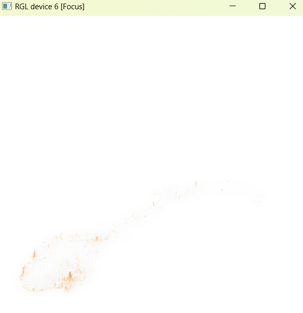
)The result appear in a RGL device and looks like Figure 1. Nothing amazing so far. This is just an interactive device where we can explore our plot.
5.2 Render camera
When we have our plot rendered, we can play with the zoom, theta and phi angles by using the render_camera function. This is very convenient because we don’t have to render the plot again, and it will be very fast:
render_camera(
zoom = 0.35,
theta = 10,
phi = 15
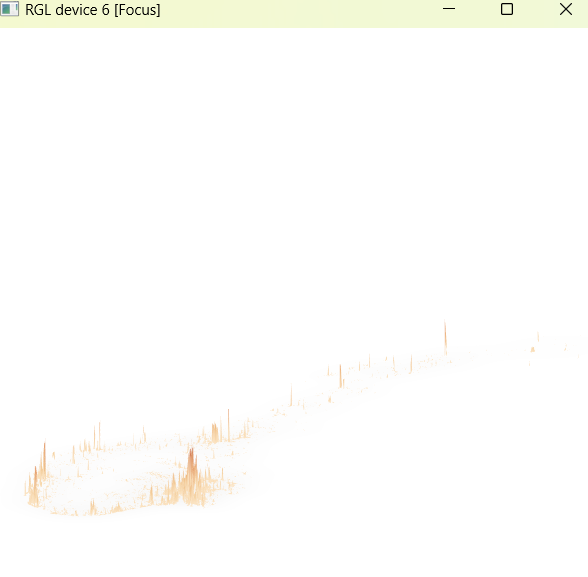
)After playing for a while with the values I decided to keep these values as my final choice, which correspond to the Figure 2.
5.3 Render in high quality
When we have our RGL device with our desired map, we can render it to a high quality image.
Note
This is very computational expensive, and depending on the specifications of your machine this process may fail for higher resolutions
Note that for a size of 2,000 it takes around 5 minutes to run in my computer. However, with a size of 6,000 it takes over 30 minutes. Here I use the function render_quality() with the following arguments:
Preview: whether or not to preview how the object is rendered (it gives a hint of the remaining time to finish).
Lightdirection: angle(s) of direction from where the sun is lightening our map.
Lightaltitude: angle(s) of altitude of the sun from the horizontal surface.
Lightintensity: intensity of the light(s).
Lightcolour: colour of the light(s).
Interactive: whether the scene will be interactive.
Width and height: defines the resolution of the resulting image.
rayshader::render_highquality(
  filename       = "norway_spikes_map.png",
  preview        = TRUE,
  light          = TRUE,
  lightdirection = c(240, 320),
  lightaltitude  = c(20, 80),
  lightintensity = c(600, 100),
  lightcolor     = c(lighten(pal[7], 0.75), "white"),
  interactive    = FALSE,
  width          = dim(population_stars)[1],
  height         = dim(population_stars)[2]
)
The resulting image (using a size of 6,000 and zscale of 20) is shown in Figure 3.
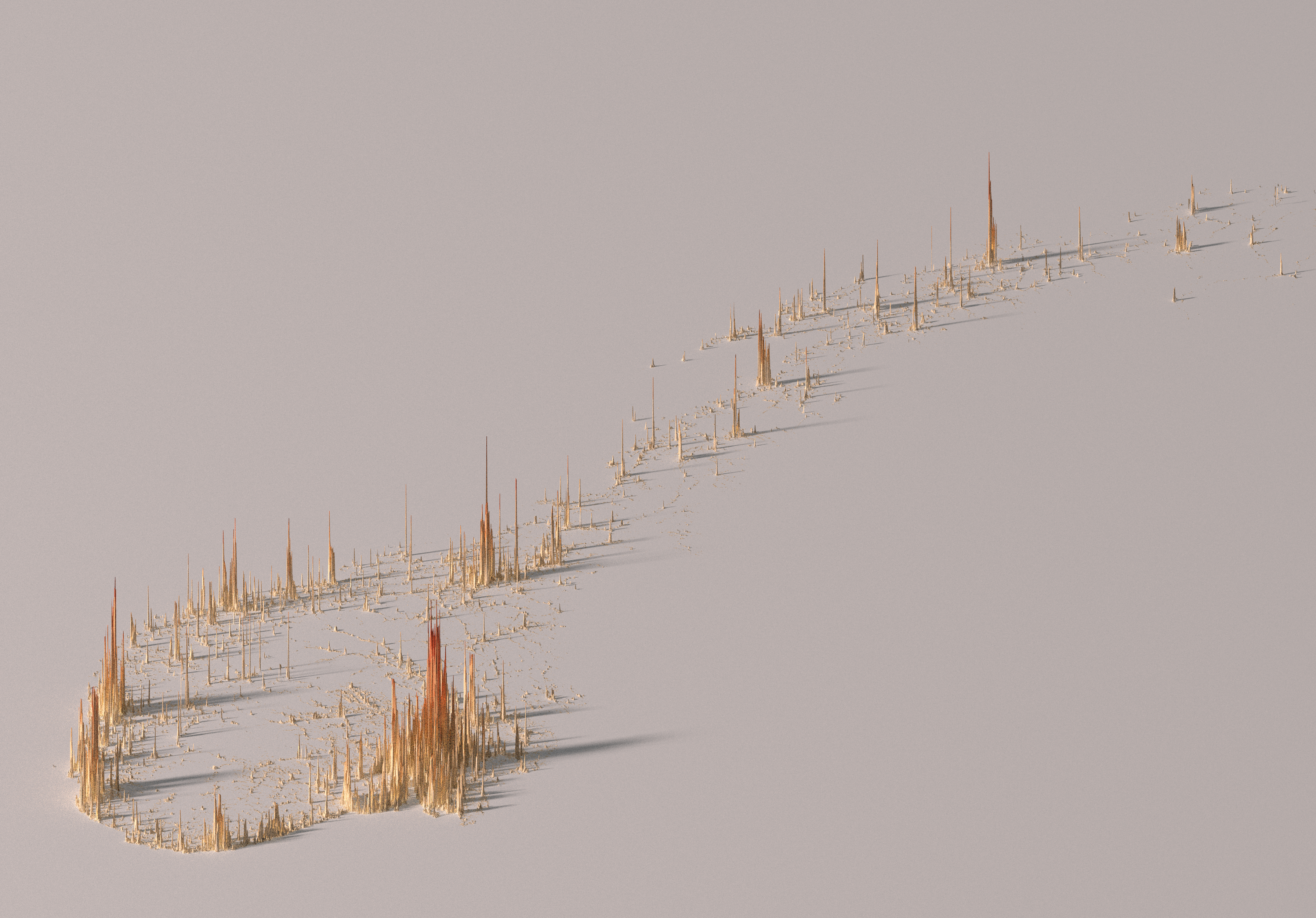
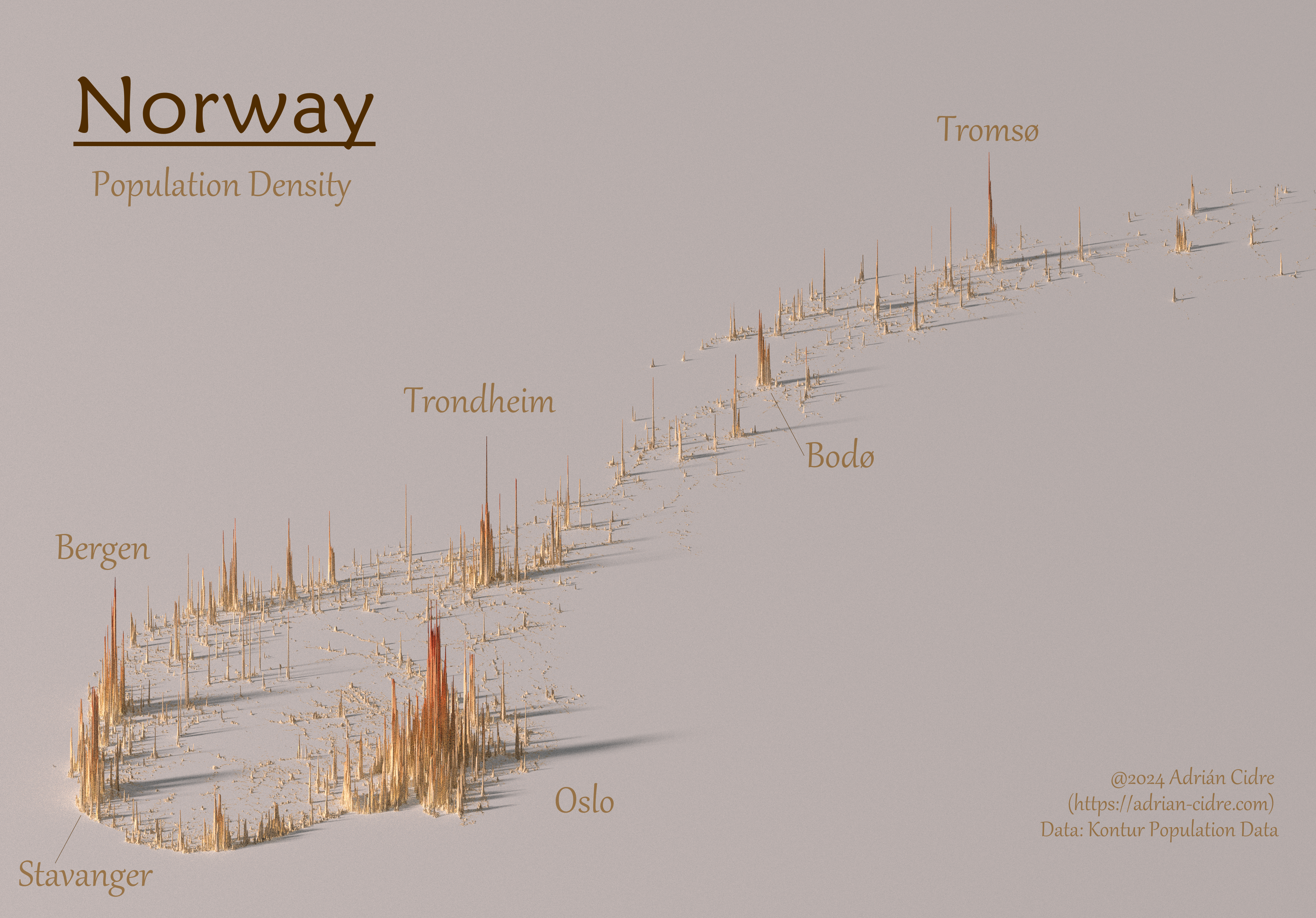
We can see that most of the population of Norway in the half south of the country, specially in Viken region. We can also add some labels to the map, so we get the final result in Figure 4.