There’s a new duck in the R pond! The first one I raised was {duckspatial}, and the newest to join him goes by {duckh3}.
What does this one bring? {duckh3} wraps the H3 community extension for DuckDB and follows the same design principles as {duckspatial} — but before diving in, let’s talk about what H3 actually is.
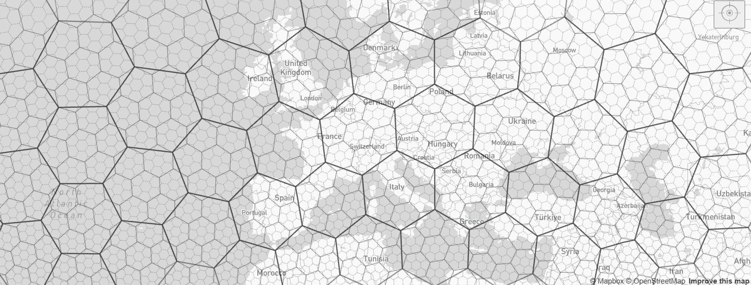
H3 is a hierarchical hexagonal grid system developed by Uber and released as open source in 2018. It divides the entire surface of the Earth into hexagonal cells at multiple resolutions: from coarse (resolution 0, ~4,250 km² per cell) to fine (resolution 15, ~0.9 m² per cell). Each cell is identified by a unique 64-bit integer index, which makes spatial operations extremely fast and storage-efficient.
Figure 1: Screenshot of the H3 grid system (source: h3geo).
Why hexagons? Unlike squares or triangles, hexagons have a unique geometric property: every neighbor is equidistant from the center, which eliminates the diagonal-vs-cardinal distance bias that plagues square grids. This makes them ideal for spatial aggregation, movement modeling, and proximity analysis. The H3 system is particularly useful when you need to:
Aggregate point data (e.g., GPS pings, sensor readings) into uniform spatial units
Join datasets from different sources without complex polygon overlaps
Analyze spatial patterns at multiple scales by moving between resolutions
{duckh3} provides fast, memory-efficient functions for analysing and manipulating large spatial and non-spatial datasets using the H3 hierarchical indexing system in R. It bridges DuckDB’s H3 extension with R’s data and spatial ecosystems — in particular {duckspatial}, {dplyr}, and {sf} — so you can leverage DuckDB’s analytical power without leaving your familiar R workflow. You can find the package’s repository here.
Let’s load some packages to introduce this {duckh3}.
Load packages
library(arrow) # parquet formatlibrary(dplyr) # data wranglinglibrary(duckdb) # interface with duckdblibrary(duckh3) # duckdb h3 extensionlibrary(duckspatial) # duckdb spatial extensionlibrary(mapgl) # interactive mapslibrary(sf) # vector data
2 Naming conventions
All functions follow the ddbh3_*() prefix (DuckDB H3), structured around the expected input data, and what they will be converted to:
ddbh3_lonlat_to_*() — from longitude/latitude coordinates to H3 representations
ddbh3_points_to_*() — from spatial point geometries to H3 representations
ddbh3_h3_to_*() — convert H3 cells to other representations
ddbh3_vertex_to_*() — convert H3 vertexes to other representations
With the following available transformations:
Function family
Output
*_to_h3()
H3 index as string or UBIGINT
*_to_spatial()
H3 cell as spatial hexagon polygon
*_to_lon()
Longitude of H3 cell centroid
*_to_lat()
Latitude of H3 cell centroid
And there are also a set of function to retrieve or check properties of the data:
ddbh3_is_*() — check properties of H3 indexes (valid, pentagon, Class III…)
The functions might be slightly verbose, but we sacrificed that in order to make them very intuitive and descriptive.
3 First steps
There are several options to work with {duckh3}, but the main two options are:
Interacting with a DuckDB connection: we won’t explain this, but if you want more details you can explore this post about {duckspatial}, as the framework is the same). There’s a convenient function to create a connection with all the setup (ddbh3_create_conn()).
Working entirely in R: the functions of this package work with lazy-tables (i.e. tables that live in a DuckDB database, and they are not materialized into R until explicitly called). This makes the processing of the data more efficient, as the data doesn’t need to be in the R’s memory until all the processing within DuckDB is done. We will focus on this workflow.
So after we have loaded the package into the R session, we need to setup the environment with the ddbh3_default_conn() function. This will:
Create a default in-memory DuckDB’s connection that will be used internally by the package.
Optionally set the maximum number of threads and RAM allowed to use by {duckh3}. By default, DuckDB will use all the available cores and 80% of RAM.
ddbh3_default_conn()
For the moment this will be a mandatory step at the beginning of the script before using any {duckh3} function.
4 Example data
For the examples below, I will use the Burnt Area database from the EFFIS, which is a database that contains data about the wildfires that happened in Europe from 2016 until the current date (April 2026). I have prepared the data previously, and simplified it for the examples. The data contains six columns:
year: the year of the wildfire
country: the 2-letter ISO code of the country
area_ha: the amount of hectares the wildfire burned
lon: the geographic longitude of the centroid of the final perimeter
lat: the geographic latitude of the centroid of the final perimeter
It’s not perfect, but it will be do for the examples. Let’s start opening the data and exploring it:
We have a total amount of 96421 wildfires during the 10-year period. Let’s assign an H3 index to each pair of coordinates. For the sake of the exercise, let’s use an H3 resolution of 4, which is about 1,770 km2.
## Add H3 as a new columnwildfires_h3_tbl <-ddbh3_lonlat_to_h3(wildfires_tbl, resolution =4)wildfires_h3_tbl
The table is lazy: it was inserted in the default’s DuckDB connection, and it’s living there.
A new column with a default’s name h3string was added.
If we work with the default names that the package use, we save some writing. For example, the default names for longitude and latitude are lon and lat, so we don’t need to specify those argument. If our columns had a different name we should specify them.
The object is not spatial. We just added the h3strings, but we didn’t convert the data to spatial. We have the functions that end in _to_spatial() to do so.
5 Analysis with duckh3
One typical analysis that we can do with the H3 grid system, is to aggregate values by the hexagons. Let’s calculate the total burned area during the 10-year period in the hexagons that we defined:
## Calculate total area by H3wildfires_agg_tbl <- wildfires_h3_tbl |>summarise(area_ha =sum(area_ha, na.rm =TRUE),.by = h3string )wildfires_agg_tbl
That’s amazing!! There we just saw a couple of functions of the package, but you see the pattern. You have a bunch of more examples in the functions documentation, and hopefully, I will add some vignettes soon to the package.
6 Low-level processing
The package also offers low-level processing. For example, let’s obtain the resolution of the following two H3 strings:
Of course, {duckh3} is not the only choice out there to work with the H3 grid system in R. Other popular options are:
{h3}: it has a very basic integration with {sf}. It’s simple and lightweight, but it has several limitations when working with spatial data. It’s not in CRAN currently.
{h3jsr}: one of the most popular options nowadays with the higgest number of downloads from CRAN. Its integration is via JavaScript and it’s integrated with current’s R ecosystem. It’s great for smaller datasets, but it’s weak when working with millions of observations.
{h3r}: implements the H3 grid system using C through the R package {h3lib}. It provides a low-level API without integration with {sf}.
{h3o}: a new R package written in Rust, that is very fast, it has a strong integration with the current geospatial ecosystem in R and the {tidyverse}, and it’s very R-user friendly.
{duckh3}: it uses DuckDB to speed up the workflows, it has a strong integration with the current geospatial ecosystem in R and the {tidyverse}. It provides processing at the table level, and vector level. It’s complemented with {duckspatial} for spatial data workflows.
8 Supporting duckh3
You can support this project by:
Trying the package, and staring the project in GitHub if you find it useful.
This development of this package wouldn’t be possible without the incredible work of many people.
First and foremost, my deepest thanks to the DuckDB team for building such a powerful and elegant analytical engine. Their commitment to performance, correctness, and developer experience has created a foundation that makes tools like {duckspatial} and {duckh3} possible. This includes the developers and maintainers of the duckdb R package, which makes possible to operate with this awesome tool from R, and it makes possible to create packages such as {duckh3}.
Special recognition goes to the developers of the DuckDB H3 Extension, the engine that powers everything in {duckh3}. Their invaluable work on spatial operations, format support, and performance optimization is what makes this package capable of handling large-scale spatial analysis efficiently.
Most importantly, this package represents a true collaborative effort. Rafael Pereira and Egor Kotov have been fundamental in shaping the design of {duckspatial}, and consequently, the design of {duckh3}.
Finally, thank you to the broader R spatial community for building the ecosystem that {duckspatial} and {duckh3} integrates with, and to everyone who has tested early versions, reported issues, or provided feedback.
10 Session Information
Analyses were conducted using the R Statistical language (version 4.6.0; R Core Team, 2026) on Windows 11 x64 (build 26200), using the packages duckh3 (version 0.1.0; Cidre González A et al., 2026), duckspatial (version 1.0.0.9000; Cidre González A et al., 2026), duckdb (version 1.5.2; Mühleisen H, Raasveldt M, 2026), sf (version 1.1.0; Pebesma E, Bivand R, 2023), DBI (version 1.3.0; R Special Interest Group on Databases, R-SIG-DB), arrow (version 23.0.1.2; Richardson N et al., 2026), mapgl (version 0.4.6; Walker K, 2026) and dplyr (version 1.2.1; Wickham H et al., 2026).
Cidre González A, Kotov E, Pereira R (2026). duckspatial: R Interface to ‘DuckDB’ Database with Spatial Extension. R package version 1.0.0.9000, commit 10cd2fb24c2750be999658b73a45ee9fd3d45d38, https://github.com/Cidree/duckspatial.