## Load pacman
library(pacman)

## Load rest of the packages
p_load(geodata, giscoR, mapboxapi, mapgl, sf, terra, tidyverse)Density interactive map of wolf in the Iberian Peninsula
1 Introduction
Today we will see how to create a map of the density of wolves’ observations in the Iberian Peninsula during the last decade (2014-2023).
We will use data from the Global Biodiversity Information Facility (GBIF) through the {geodata} package, and we will create an interactive heatmap using the new {mapgl} R package.
2 Loading packages
We will use the following packages:
{geodata}(Hijmans et al. 2024): we will use it to download data from the GBIF database.{giscoR}(Hernangómez 2024): to download the boundaries of the study area.{mapboxapi}(Walker 2024): to store our mapbox API access token.{mapgl}(mapgl): to create the interactive maps. The package is not published in CRAN yet.{sf}(Pebesma and Bivand 2023): to manipulate vectorial data.{terra}(Hijmans 2024): to manipulate raster data.{tidyverse}(Wickham et al. 2019): to manipulate data in general.
3 Mapbox API
Mapbox is an online maps provider that is currently used by many companies in the world, and it’s accessible through R using the {mapgl} package. You can create an account for free in https://www.mapbox.com/, so you can get your API token.
Note that mapbox will ask you for your billing address at any time, because this service is not completely free. But don’t worry, for this tutorial you won’t be charged.
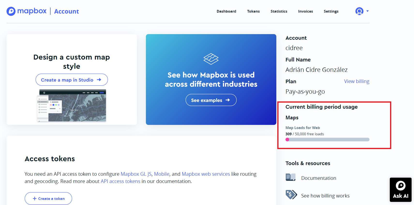
Once you created your account, you can log in into the mapbox webpage, and you will see something like this:
On the right side, you can see the current billing period usage. You can have up to 50,000 map loads per month for free, but when you surpass this number you’ll be charged (more details about pricing here).
Note that every view triggers a map load
So, if you want to continue with this tutorial, you must create an API access token in your mapbox dashboard Figure 1. Once you have your token, you have two options to use it:
This option will work only for the current project. You will use the following function which will use a .Renviron file to store and access the token:
mb_access_token("your_token_goes_here", install = TRUE)After executing this line of code, you must restart you R session to take effect.
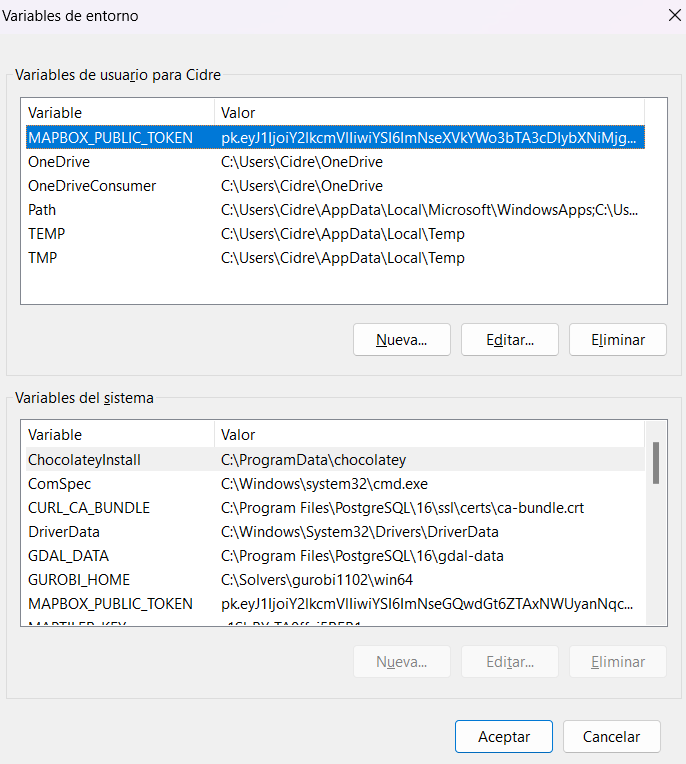
This option will store the API token as an environment variable in your system, and it can be accessed by any project in your computer. Find your environment variables, and create a new one called MAPBOX_PUBLIC_TOKEN with the value of your token:
After you’ve done this, you need to close and open Rstudio to take effect.
Note that you should never share your token with anybody. In the case that your token has been compromised, delete it and create a new one.
4 Load the data
In this exercise we need to download two sources of data, that we already used in the previous week’s post:
Study area
Wolf data
4.1 Study area
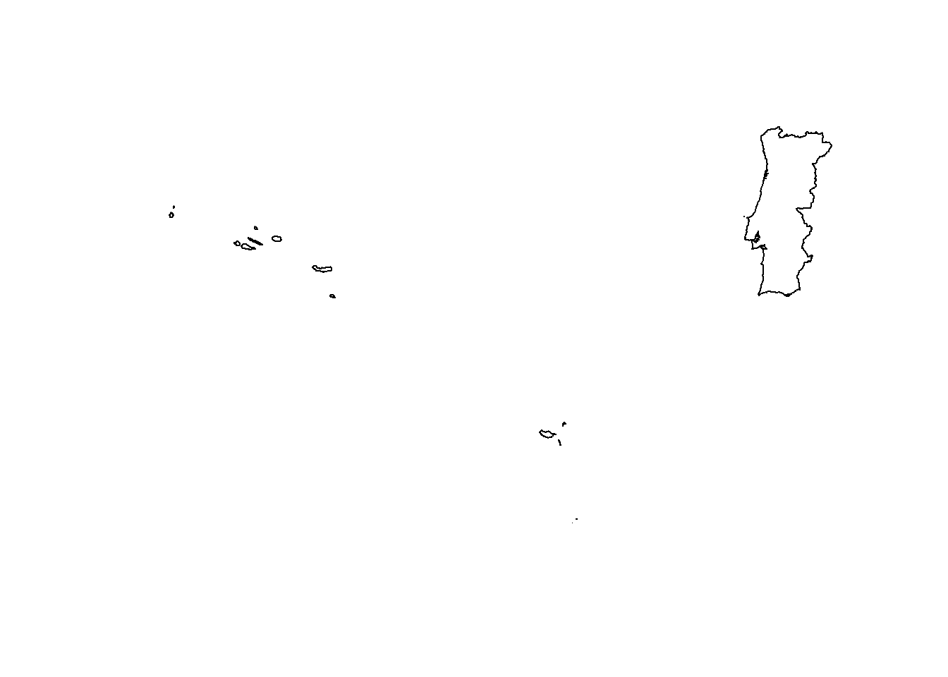
The study area for this exercise is the Iberian Peninsula, which includes the main land of Spain and Portugal without islands. To extract this area, we need first to get the boundaries of Spain and Portugal, eliminate the islands, and combine both countries. So, one step at a time. We start downloading the country of Portugal, and casting the MULTIPOLYGON to POLYGON:
## Get Portugal
portugal_sf <- gisco_get_countries(
  resolution = "01",
  country    = "Portugal"
) |>
  st_cast("POLYGON")

## Visualize
plot(st_geometry(portugal_sf))To filter the main land, we can calculate the area of each polygon, and slice the polygon with the maximum value of area:
## Get main land
portugal_sf <- portugal_sf |>
  mutate(
    area = st_area(portugal_sf)
  ) |>
  slice_max(area)

## Visualize
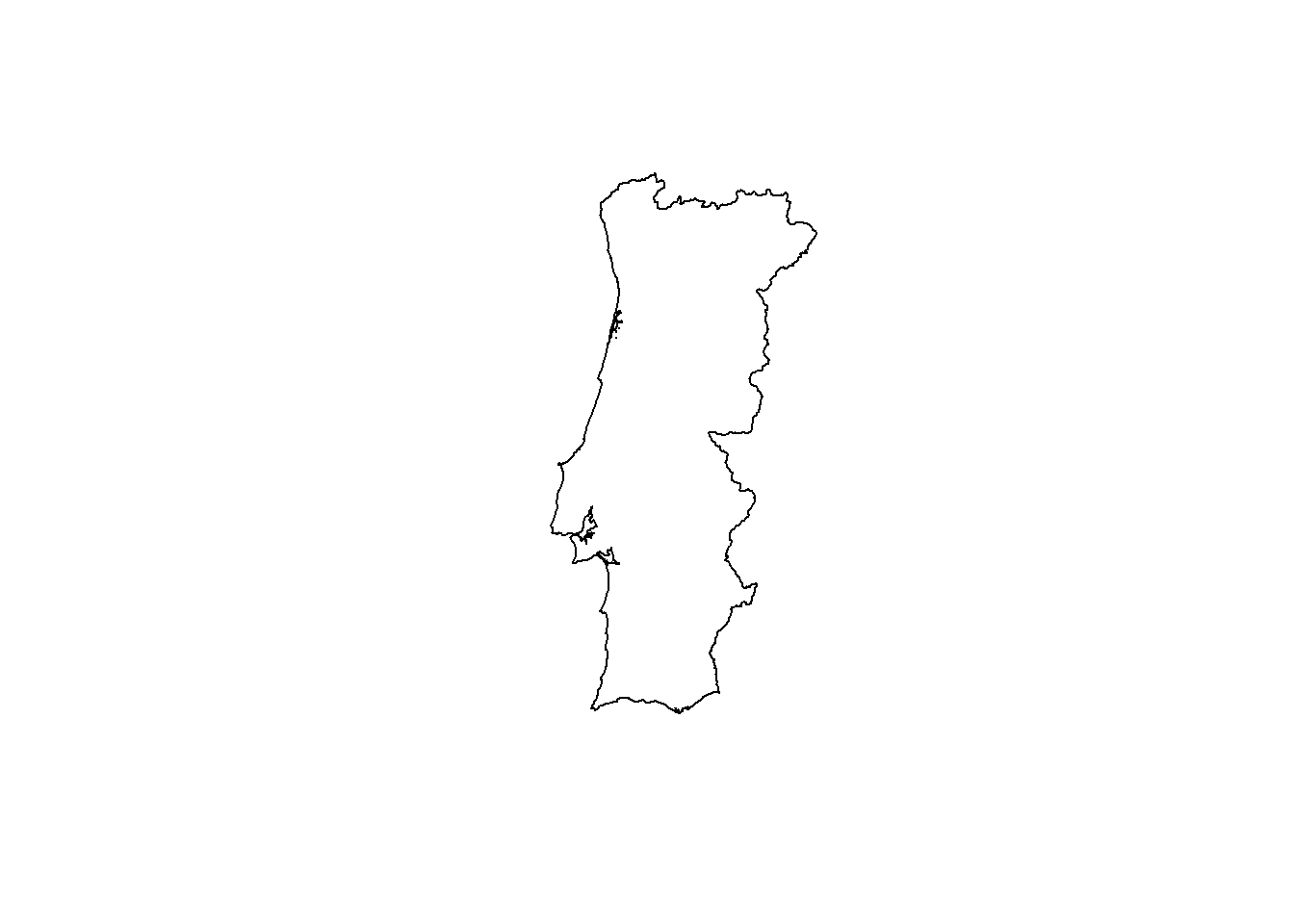
plot(st_geometry(portugal_sf))Now, we can do the same for Spain:
## Get Spain
spain_sf <- gisco_get_countries(
  resolution = "01",
  country    = "Spain"
) |>
  st_cast("POLYGON")

## Get main land
spain_sf <- spain_sf |>
  mutate(
    area = st_area(spain_sf)
  ) |>
  slice_max(area)

## Visualize
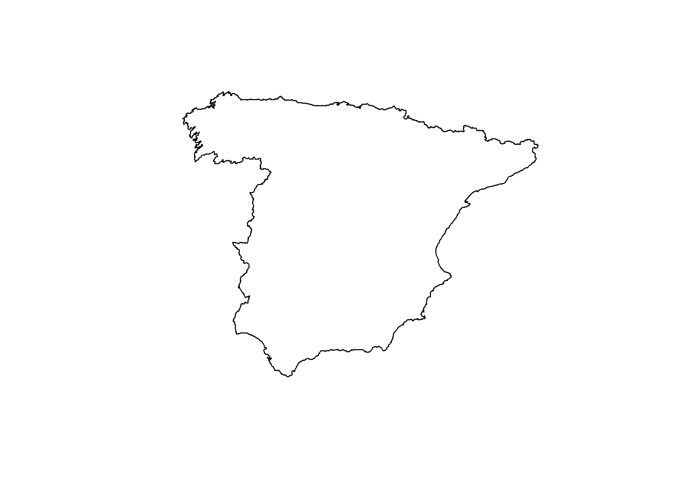
plot(st_geometry(spain_sf))Up to this point, we have two different {sf} objects with the main land of Portugal Figure 3 and Spain Figure 4. The final step, is to combine them to form only one polygon:
## Make union
iberia_sf <- st_union(
  spain_sf,
  portugal_sf
) |>
  st_transform(25830)

## Visualize
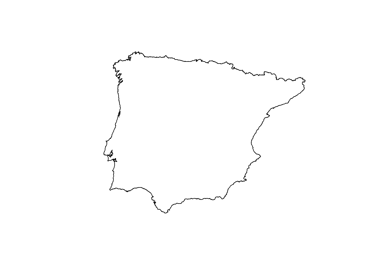
plot(st_geometry(iberia_sf))Note that we also transformed the Coordinates Reference System to a projected system (EPSG 25830).
4.2 Wolf data
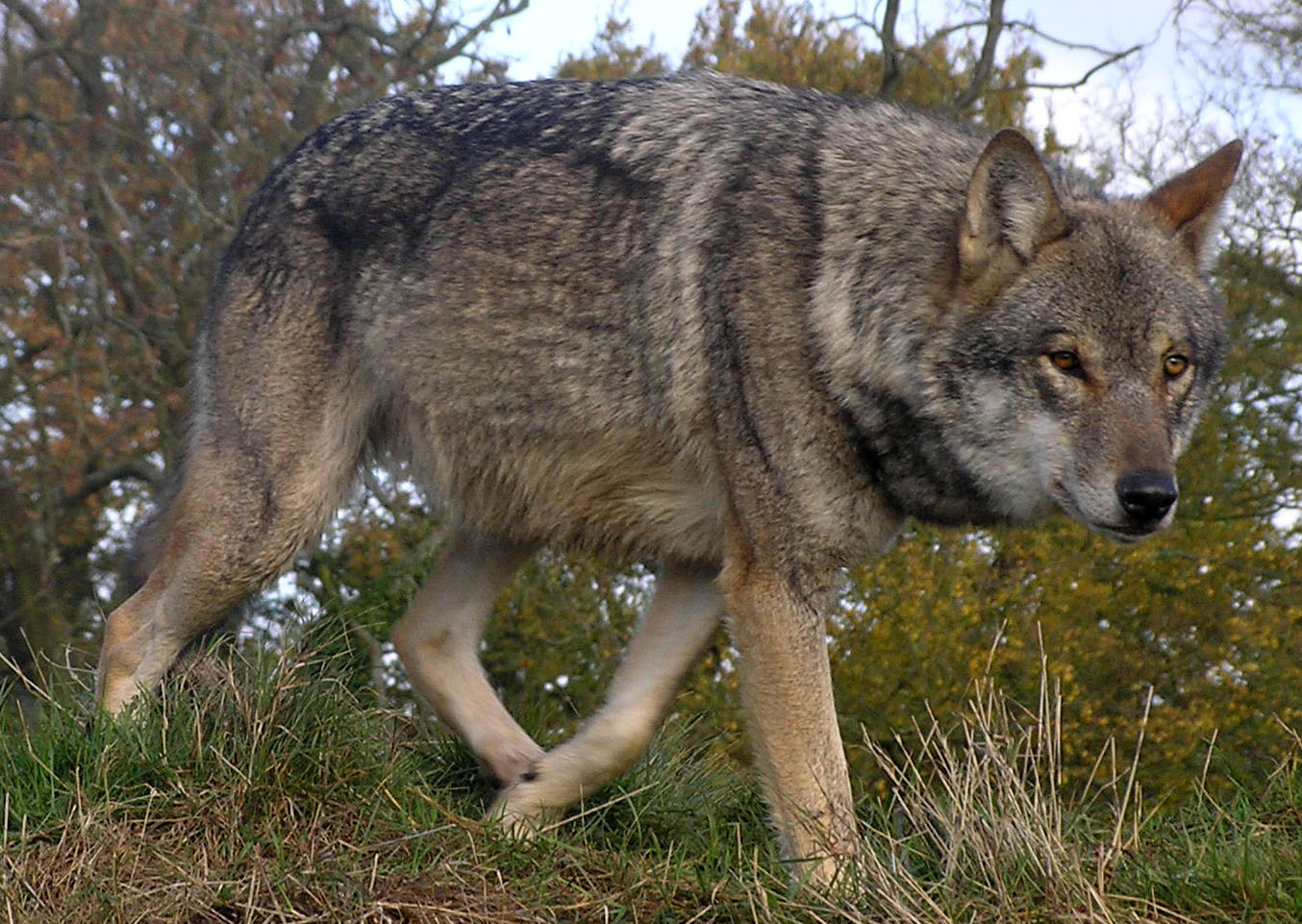
In this exercise, we will study the distribution of the gray wolf (Canis lupus; Figure 6) in the Iberian Peninsula:
As a proxy of the distribution, we will use data from GBIF for the period 2014-2023. This database contains information about observations of any species in the world. We will use the sp_occurrence() function from the {geodata} package, and we will add two arguments to specify the countries (ES for Spain, PT for Portugal) and the period (2014-2023).
To specify a period, separate two years by a comma.
## Download wolf data
## - Years: 2014-2023
wolf_lst <- map(
  .x = c("ES", "PT"),
  .f = \(x) sp_occurrence(
    genus   = "Canis",
    species = "lupus",
    args    = c(
      paste0("country=", x),
      "year=2014,2023"
    )
  )
)
Note that we use the purrr::map() function to iterate over two elements (ES and PO) which are used in the country argument.
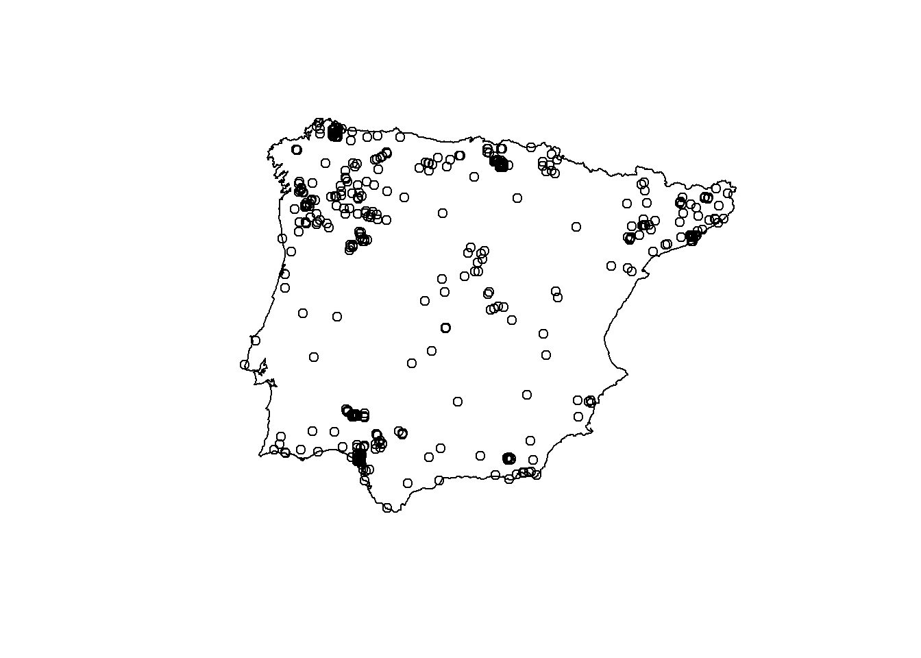
We are using a projected CRS, but the coordinates data that we have in wolf_lst are in the WGS 84. Therefore, we need to transform this list to a sf object, and transform the coordinates to the new CRS.
Another thing to note is that we have data from the entire countries, but we want only from the Iberian Peninsula. In this sense, we can use st_intersection() to filter only the observations in the Iberian Peninsula.
## Bind data, convert to sf, transform and select points within Iberia
wolf_sf <- list_rbind(wolf_lst) |>
  st_as_sf(
    coords = c("lon", "lat"),
    crs    = 4326
  ) |>
  st_transform(25830) |>
  st_intersection(iberia_sf) |>
  select(country)

## Visualize
plot(st_geometry(wolf_sf))
plot(st_geometry(iberia_sf), add = TRUE)5 Introduction to mapgl
Before creating the heatmap, we will see how to use the functions of this package. If you followed the Section 3, you can run the following code to create a basic mapbox map:
mapboxgl()You can zoom in and out in the map, and you can also use your right mouse button to rotate the map. If you zoom in to a city, you will see some of the buildings in 3D, which I think it’s amazing!!
Now, we will tweak some parameters:
mapboxgl(
  style  = mapbox_style("satellite"),
  center = c(-7, 42),
  zoom   = 5
) |>
  fly_to(
    center = c(-7, 42),
    zoom   = 10
)- style: this argument takes the function
mapbox_style()to set a base map. The possible options are: standard, streets, outdoors, light, dark, satellite, satellite-streets, navigation-day, and navigation-night. - center: the coordinates of the center of the map in the beginning.
- zoom: the zoom level of the map in the beginning.
- fly_to(): this function will create a flying effect from the center and zoom set in the
mapboxgl()function to the ones selected infly_to().
6 Wolves heatmap
Finally, we will create a heatmap of the density of wolves in the Iberian Peninsula. We will add the layer to the map using the add_heatmap_layer() function which takes the following mandatory arguments:
id: an unique ID for the layer
source: the data source. In this case, an
sfobject.
There are other optional arguments that can improve the map:
- heatmap_opacity: the opacity of the heatmap layer. 0 is completely transparent, 1 is completely opaque.
- heatmap_intensity: defines the intensity of the points. An interpolation expression can be used to define the intensity.
- Other arguments: heatmap_color, heatmap_radius, heatmap_weight …
An interpolation expression is an expression which smoothly transitions values between a series of stops.
mapboxgl(
  style = mapbox_style("satellite")
) |>
  fit_bounds(
    iberia_sf
  ) |>
  add_heatmap_layer(
    id     = "wolves-heatmap",
    source = wolf_sf,
    heatmap_intensity = interpolate(
      property = "heatmap-density",
      values   = c(0, 1),
      stops    = c(1, 2)
    ),
    heatmap_opacity = .5
  )
Note that we also used the fit_bounds() function to fit the map view to the extent of the Iberian Peninsula.
7 Conclusions
Currently, there are many different packages allowing you to create interactive maps in R (mapview, leaflet, plotly, mapboxapi, mapgl …). I think mapgl is great because it let us to create interactive maps using mapbox, which can load faster and more data than other alternatives. Note also that this package it’s in early stages and might have some limitations, and new features to come.
However, as you could see, mapbox it’s not completely free and that might be a limitation for some users. In this sense, MapLibre has appeared as fork of mapbox which is completely free and it can also be used through the {mapgl} package. The next week, we will cover more features of this package using MapLibre.
