library(pacman)

p_load(
  ## Data manipulation
  tidyverse, readxl,

  ## Spatial data manipulation
  sf,

  ## Download data
  mapSpain,

  ## Visualization
  rayshader
)Spanish Burned Area during 2006-2015 by Municipality
R
forestry
wildfires
ggplot2
rayshader
Creating a 3D visualization of the burned area in Spain by municipality during the period 2006-2015 using {rayshader}.
1 Introduction
In this post, we will explore the distribution of the burned area in Spain by municipality creating a 3D visualization using the awesome package {rayshader} 😎.
Honestly, I am not fan of 3D plots in general, because they are usually horrible and deceiving when trying to communicate something. However, with {rayshader} we can create spikes maps which can somehow look great and communicating the message properly.
Important
If you can, avoid always to create a 3D plot (3D pie charts (even 2D, please), 3D bar charts…).
The data was obtained from the MITECO (Ministerio para la Transición Ecológica y el Reto Demográfico), and it can be found in this url.
I will use the data for the decade 2006-2015, which is the latest available data for this purpose.
2 Loading packages
As usually, we will start loading all the necessary packages by using the {pacman} package.
We will use the {tidyverse} for data wrangling and visualization, the {readxl} package for reading our data in Excel format, the {sf} package for vectorial data manipulation, the package {mapSpain} for downloading some convenient spatial data, and finally {rayshader} for creating 3D visualizations.
3 Load the data
The data is the same I used in the previous post, but this time we will work with the municipalities instead of autonomous communities, and with burned area instead number of wildfires. Nevertheless, the first step will be to load the data, and fix the table names so we can all understand what’s going on with this dataset:
## Load data
wildfires_tbl <- read_excel("wildfires_2006_2015.xlsx", sheet = 3)

## Set names
wildfires_tbl <- wildfires_tbl %>%
  select(
    mun = NOMBRE, code = CODIGOINE, woodland_area = ARBOLADO,
    treeless_area = NOARBOLADO, total_area = TOTAL
  )

glimpse(wildfires_tbl)
Rows: 4,376
Columns: 5
$ mun <chr> "A Arnoia", "A Baña", "A Bola", "A Cañiza", "A Capela", …
$ code <dbl> 32003, 15007, 32014, 36009, 15018, 15030, 36017, 27018, …
$ woodland_area <dbl> 30, 615, 16, 978, 394, 18, 262, 600, 8, 803, 30, 364, 60…
$ treeless_area <dbl> 8, 82, 61, 1260, 165, 104, 791, 641, 17, 3395, 6, 1558, …
$ total_area <dbl> 38, 697, 77, 2238, 559, 122, 1053, 1241, 25, 4198, 36, 1…I selected a total of 5 columns: the first two columns corresponds to the name and ID of the municipalities, and the remaining columns refer to the burned area (woodland, treeless, and total burned area).
4 Prepare data
The data preparation is not very demanding to be honest. We have to download the map of Spain by municipalities, and for doing so, we have the convenient function esp_get_munic() from the {mapSpain} package:
## Get data
esp_mun_sf <- esp_get_munic() %>%
  filter(!(ine.ccaa.name %in% c("Melilla", "Ceuta"))) %>%
  mutate(code = as.numeric(LAU_CODE))

## Explore data
head(esp_mun_sf)
Simple feature collection with 6 features and 8 fields
Geometry type: POLYGON
Dimension: XY
Bounding box: xmin: -3.14019 ymin: 36.73845 xmax: -2.05701 ymax: 37.54576
Geodetic CRS: ETRS89
codauto ine.ccaa.name cpro ine.prov.name cmun name LAU_CODE
382 01 Andalucía 04 Almería 001 Abla 04001
379 01 Andalucía 04 Almería 002 Abrucena 04002
374 01 Andalucía 04 Almería 003 Adra 04003
375 01 Andalucía 04 Almería 004 Albánchez 04004
358 01 Andalucía 04 Almería 005 Alboloduy 04005
373 01 Andalucía 04 Almería 006 Albox 04006
geometry code
382 POLYGON ((-2.77744 37.23836... 4001
379 POLYGON ((-2.88984 37.09213... 4002
374 POLYGON ((-2.93161 36.75079... 4003
375 POLYGON ((-2.13138 37.29959... 4004
358 POLYGON ((-2.70077 37.09674... 4005
373 POLYGON ((-2.15335 37.54576... 4006Here, we got the Spanish map as a simple feature object from the sf package, we eliminated Ceuta and Melilla (no information about wildfires), and converted the LAU_CODE column from character to numeric.
The last step before the visualization is to join the wildfires table with the municipalities, so we have the information of the wildfires stored in a spatial object. This is pretty straightforward by using the left_join function:
esp_mun_wildfires_sf <- esp_mun_sf %>%
  left_join(
    wildfires_tbl,
    by = join_by(code == code)
  )
This will generate many NA values because in the wildfires_tbl we have a total of 4376, while in esp_mun_sf we have a total of 8129. This is because not every municipality of Spain had suffered wildfires. These NA values can be then changed by the value of 0:
esp_mun_wildfires_sf <- esp_mun_wildfires_sf %>%
  mutate(
    total_area = if_else(is.na(total_area), 0, total_area)
  )
5 2D visualization
In this post we will learn how to turn a basic {ggplot2} plot into a basic 3D visualization using {rayshader}. Therefore, the first step is to create a {ggplot2} object:
## Create ggplot2 object
esp_mun_wildfires_gg <- esp_mun_wildfires_sf %>%
  ggplot() +
  # Geometries
  geom_sf(aes(fill = total_area), color = NA) +
  # Scales
  scale_fill_distiller(palette = "Reds", direction = 1) +
  # Labels
  labs(title    = "Burned Area in Spain during 2006-2015",
       caption  = "@2023 Adrián Cidre (https://adrian-cidre.com)\nData: MITECO",
       fill     = "Area (ha)") +
  # Theme
  theme_void(base_family = "Rockwell") +
  theme(
    plot.title = element_text(
      size   = 14,
      face   = "bold",
      hjust  = .95,
      colour = "indianred4",
      margin = margin(b = 23, t = 5)
    ),
    plot.caption      = element_text(
      size   = 8,
      colour = "indianred4",
      hjust  = .5
    ),
    legend.title      = element_text(size = 8, colour = "indianred4"),
    legend.text       = element_text(size = 8, colour = "indianred4"),
    legend.position   = "bottom",
    legend.key.width  = unit(1, "cm"),
    legend.key.height = unit(0.3, "cm"),
    plot.background   = element_rect(fill = "#B0C4DE", colour = NA)
  )

## Display plot
esp_mun_wildfires_gg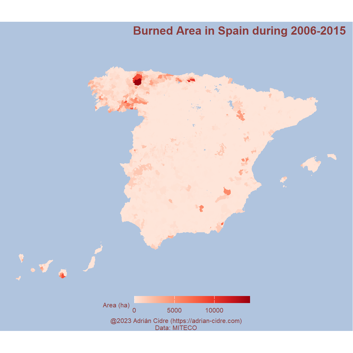
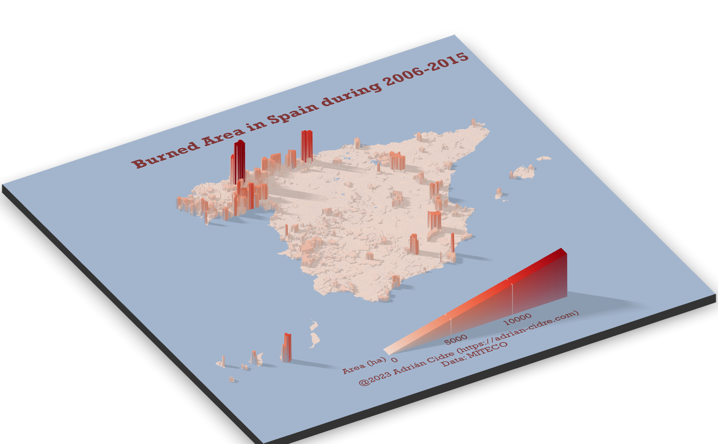
6 3D Visualization
Once we have this visualization, we can use the rayshader::plot_gg function. This function has many arguments to control the appearance of our map. In this tutorial I will show you the basic ones:
Multicore = TRUE: it will use multiple cores to compute the shadow matrix. This is computationally demanding, so this can improve the performance.
Width and height: they control the size of the
ggplot2object.Scale: the vertical scaling. The higher this number, the taller the spikes.
Shadow intensity: a number between 0 and 1, representing the intensity of the shadows. When set to 0 the shadows are completely black, while 1 means no shadows.
Sunangle: the angle from where the sun would generate the shadows. The default 315, means that the sun is shining from the North West.
Offset edges: when TRUE, adds some space between polygons.
Window size: the size of the RGL device (preview window) when executing the function.
Zoom: amount of zoom to the plot.
Phi (\(\phi\)): azimuth angle (Figure 2).
Theta (\(\theta\)): rotation around z-axis (Figure 2).

With all these parameters set, we can execute the function plot_gg() which will open a new window to visualize the rendered plot:
plot_gg(
  esp_mun_wildfires_gg,
  multicore        = TRUE,
  width            = 5,
  height           = 5,
  scale            = 150,
  shadow_intensity = .6,
  sunangle         = 315,
  offset_edges     = FALSE,
  windowsize       = c(600, 600),
  zoom             = .5,
  phi              = 35,
  theta            = -30
)
After we set the parameters that makes us happy, we can export the last rendered object by using the rayshader::render_snapshot() function:
render_snapshot(filename = "wildfires_ha_muni.png", clear = FALSE)The result can be seen in Figure 3. As we saw in my previous post, the area that is most affected by the wildfires is by far the northwestern area of Spain, both in number of fires and burned hectares.