library(pacman)

p_load(
  ## Core
  tidyverse, readxl, stringi,

  ## Vectorial data manipulation
  sf,

  ## Download data
  mapSpain,

  ## Visualization
  RColorBrewer
)Spanish Wildfires by CCAA during 2006-2015
R
forestry
wildfires
ggplot2
Exploring the distribution of the forest wildfires in Spain by Autonomous Community, creating some descriptive graphs using R and ggplot2.
1 Introduction
In this post, we will explore the distribution of the forest wildfires in Spain by Autonomous Community, creating some descriptive graphs using R and {ggplot2}.
The data was obtained from the MITECO (Ministerio para la Transición Ecológica y el Reto Demográfico), and it can be found in this link.
I will use the data for the decade 2005-2015, which is the latest available database for this purpose.
2 Loading packages
First, we will load some packages:
Here, I will use the {tidyverse} as usual for data analysis and visualization, the package {readxl} since the data is in Excel format, and {stringi} for some string manipulation. Then, the package {sf} for vectorial data manipulation, {mapSpain} to download the map of Spain by any NUTS level. Finally, I will use {RColorBrewer} for colour palettes.
3 Data exploration
Once the packages are loaded, we can load the data. Note that the data is on the \(3^{rd}\) sheet of the Excel file. The variables are in Spanish, so I will change some names to English so we can all understand what’s going on.
## Load the data
wildfires_tbl <- read_excel("wildfires_2006_2015.xlsx", sheet = 3)

## Set new names
wildfires_tbl <- wildfires_tbl %>%
  select(municipality = NOMBRE, ccaa = COM_N_INE, small_fires = conatos, wildfires = incendios,
         total_wildires = TOTAL_INCENDIOS, woodland_area = ARBOLADO,
         treeless_area = NOARBOLADO, total_area = TOTAL)

## Overview of the data
glimpse(wildfires_tbl)
Rows: 4,376
Columns: 8
$ municipality <chr> "A Arnoia", "A Baña", "A Bola", "A Cañiza", "A Capela",…
$ ccaa <chr> "Galicia", "Galicia", "Galicia", "Galicia", "Galicia", …
$ small_fires <dbl> 27, 66, 74, 330, 12, 149, 156, 75, 33, 426, 30, 58, 86,…
$ wildfires <dbl> 3, 37, 12, 81, 6, 24, 54, 47, 4, 273, 3, 62, 28, 16, 28…
$ total_wildires <dbl> 30, 103, 86, 411, 18, 173, 210, 122, 37, 699, 33, 120, …
$ woodland_area <dbl> 30, 615, 16, 978, 394, 18, 262, 600, 8, 803, 30, 364, 6…
$ treeless_area <dbl> 8, 82, 61, 1260, 165, 104, 791, 641, 17, 3395, 6, 1558,…
$ total_area <dbl> 38, 697, 77, 2238, 559, 122, 1053, 1241, 25, 4198, 36, …So we can see that there is data about the number of wildfires, and the area burned. This week we will study the number of wildfires and the next week we will have a look to the area burned and their relationship.
There are a total of 4,376 observations, where each observation stands for a single municipality (therefore, the column municipality can be thought as the ID). Then, we have the Autonomous Community (ccaa) to which the municipality belongs, the number of fires, and the burned area. To those who are not familiarized with the concept of “conato”, which I translated as small fire, this is:
Conato: wildfires where the total burned area is less than 1 hectare. This definition applies to the data here; however, in some Autonomous Communities the definition may be different. For instance, in Galicia they consider that less than 0.5 hectares must be woodland area, otherwise, it is categorized as normal wildfire.
There is also another category called Grandes Incendios Forestales (Large Forest Fires), which are those that burn more than 500 hectares. However, they did not consider this category in the data.
NoteNote
If you are interested, the first two sheets of the Excel file contain some metadata and information about the variables.
4 Analysing the number of wildfires
Let’s do some data wrangling! Since we will analyse the wildfires by Autonomous Community, we need to summarise our data using the ccaa variable. So this can be easily done as follows:
wildfires_ccaa_tbl <- wildfires_tbl %>%
  group_by(ccaa) %>%
  summarise(
    total_wildfires = sum(total_wildires)
  ) %>%
  ungroup()

wildfires_ccaa_tbl
# A tibble: 17 × 2
ccaa total_wildfires
<chr> <dbl>
1 Andalucia 7519
2 Aragon 3055
3 Canarias 954
4 Cantabria 6257
5 Castilla y Leon 16421
6 Castilla-La Mancha 6725
7 Cataluña 3751
8 Comunidad Foral de Navarra 4577
9 Comunidad de Madrid 2657
10 Comunitat Valenciana 3349
11 Extremadura 8148
12 Galicia 37870
13 Illes Balears 1031
14 La Rioja 634
15 Pais Vasco 913
16 Principado de Asturias 16979
17 Region de Murcia 1157Cool. This starts to look pretty good, but we need to apply some formatting. First, we can order the Autonomous Communities by descending order of the total wildfires, and create a label with the percentages format.
wildfires_ccaa_total_tbl <- wildfires_ccaa_tbl %>%
  mutate(
    ccaa       = fct_reorder(ccaa, total_wildfires),
    label_perc = scales::percent(total_wildfires / sum(total_wildfires),
                                 accuracy = .01)
    ) %>%
  arrange(desc(total_wildfires))

wildfires_ccaa_total_tbl
# A tibble: 17 × 3
ccaa total_wildfires label_perc
<fct> <dbl> <chr>
1 Galicia 37870 31.04%
2 Principado de Asturias 16979 13.92%
3 Castilla y Leon 16421 13.46%
4 Extremadura 8148 6.68%
5 Andalucia 7519 6.16%
6 Castilla-La Mancha 6725 5.51%
7 Cantabria 6257 5.13%
8 Comunidad Foral de Navarra 4577 3.75%
9 Cataluña 3751 3.07%
10 Comunitat Valenciana 3349 2.75%
11 Aragon 3055 2.50%
12 Comunidad de Madrid 2657 2.18%
13 Region de Murcia 1157 0.95%
14 Illes Balears 1031 0.85%
15 Canarias 954 0.78%
16 Pais Vasco 913 0.75%
17 La Rioja 634 0.52% Now this looks much better! With the function scales::percent we can do the trick to create a character column with the percentage of wildfires over the total, and with the argument accuracy we specify the decimals. The fct_reorder function is used to order the levels of the Autonomous Communities (which is necessary for visualize in this order).
Now that we have the data ready, we can create a cool visualization to explore the data better:
wildfires_ccaa_total_tbl  %>%
  head(10) %>%
  ggplot(aes(x = ccaa, y = total_wildfires)) +
  geom_col(fill = "steelblue") +
  geom_label(aes(label = label_perc)) +
  coord_flip() +
  expand_limits(y = 40000) +
  labs(x        = NULL,
       y        = "Total Wildfires",
       title    = "Wildfires by Autonomous Community (2006-2015)",
       subtitle = "Top 10 Autonomous Communities in Spain",
       caption  = "Author: Adrián Cidre González") +
  annotate(
    "rect", xmin = 7.5, xmax = 10.5, ymin = -500, ymax = 41000,
    fill = NA, color = "indianred4", lwd = 1
  ) +
  annotate(
    "text",
    x = 8.5, y = 30000,
    label = "The northwest of Spain \nsuffers the 58% of \nthe wildfires",
    color = "indianred4"
  ) +
  theme_minimal() +
  theme(plot.title = element_text(hjust = 0.5),
        plot.subtitle = element_text(hjust = 0.5))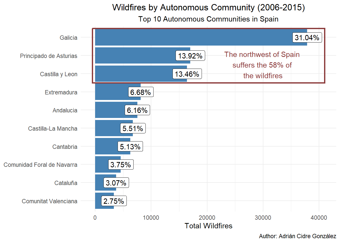
Ok, that was quite a bit of code. First, we can see that I filtered the top 10 Autonomous Communities with head. Then, we have a bar plot with the label that we previously created. The expand_limits function expands the axis so the label of Galicia can be seen properly. Next, the annotate functions create the rectangle and the label on the text. Note that we need to specify the geom of the annotation (in these cases rect and text). The rest of the arguments are just formatting. Isn’t it cool? That’s why I love {ggplot2} ❤️.
4.1 Analysing the results
There is an Autonomous Community were the number of fires are extremely high, Galicia. Almost one third of the Spanish burned area during the decade 2006-2015 was in this region, which in fact only occupies 5.8% of the territory of Spain. Next, we have Asturias with almost 14% of the total burned area, and occupying the 2.1% of the territory. To finish the top-3, we have Castilla and León where a similar area to Asturias was burned. However, Castilla and Leon is the biggest Autonomous Community of Spain representing the 18.6% of the territory. These numbers are alarming, and more when we look at the spatial location of these areas. The top-3 areas, representing the 58% of the burned area, are all located in the North-Western area of Spain.
5 Analysing the spatial distribution
To analyse the spatial distribution we need to get the vectorial data of the Autonomous Communities of Spain. One way is to use the package mapSpain:
esp_ccaa_sf <- esp_get_ccaa() %>%
  filter(!(iso2.ccaa.name.es %in% c("Melilla", "Ceuta")))
With that code I am eliminating Ceuta and Melilla, because they are not included in the wildfires dataset. The next step is to join the esp_ccaa_sf and wildfires_ccaa_total_tbl; however, there’s an issue:
esp_ccaa_sf$nuts2.name [1] "Andalucía" "Aragón"
[3] "Principado de Asturias" "Illes Balears"
[5] "Canarias" "Cantabria"
[7] "Castilla y León" "Castilla-La Mancha"
[9] "Cataluña" "Comunidad Valenciana"
[11] "Extremadura" "Galicia"
[13] "Comunidad de Madrid" "Región de Murcia"
[15] "Comunidad Foral de Navarra" "País Vasco"
[17] "La Rioja" wildfires_ccaa_total_tbl$ccaa [1] Galicia Principado de Asturias
[3] Castilla y Leon Extremadura
[5] Andalucia Castilla-La Mancha
[7] Cantabria Comunidad Foral de Navarra
[9] Cataluña Comunitat Valenciana
[11] Aragon Comunidad de Madrid
[13] Region de Murcia Illes Balears
[15] Canarias Pais Vasco
[17] La Rioja
17 Levels: La Rioja Pais Vasco Canarias Illes Balears ... GaliciaDo you see it? The names are different, so that might be a problem when we try to join them. In the wildfires dataset, they didn’t use acute accent (e.g. á). We could manually change it, but the package {stringi} allows us to this more efficiently:
esp_ccaa_sf %>%
  mutate(nuts2.name = nuts2.name %>% stri_trans_general("Latin-ASCII")) %>%
  pull(nuts2.name)
[1] "Andalucia" "Aragon"
[3] "Principado de Asturias" "Illes Balears"
[5] "Canarias" "Cantabria"
[7] "Castilla y Leon" "Castilla-La Mancha"
[9] "Cataluna" "Comunidad Valenciana"
[11] "Extremadura" "Galicia"
[13] "Comunidad de Madrid" "Region de Murcia"
[15] "Comunidad Foral de Navarra" "Pais Vasco"
[17] "La Rioja" That’s a first approach, but now we need to manually change Calatuna to Cataluña, and also Comunidad Valenciana, which was previously already different. So all the changes will be achieved as follows:
##
wildfires_ccaa_sf <- esp_ccaa_sf %>%
  mutate(nuts2.name = nuts2.name %>% stri_trans_general("Latin-ASCII")) %>%
  mutate(nuts2.name = case_when(
    nuts2.name == "Comunidad Valenciana" ~ "Comunitat Valenciana",
    nuts2.name == "Cataluna" ~ "Cataluña",
    .default = nuts2.name
  )) %>%
  inner_join(
    wildfires_ccaa_total_tbl,
    by = join_by(nuts2.name == ccaa)
  ) %>%
  select(nuts2.name, total_wildfires)

wildfires_ccaa_sf
Simple feature collection with 17 features and 2 fields
Geometry type: MULTIPOLYGON
Dimension: XY
Bounding box: xmin: -13.21924 ymin: 34.70209 xmax: 4.320511 ymax: 43.78793
Geodetic CRS: ETRS89
First 10 features:
nuts2.name total_wildfires geometry
1 Andalucia 7519 MULTIPOLYGON (((-4.275964 3...
2 Aragon 3055 MULTIPOLYGON (((-0.74093 42...
3 Principado de Asturias 16979 MULTIPOLYGON (((-4.536122 4...
4 Illes Balears 1031 MULTIPOLYGON (((4.095952 40...
5 Canarias 954 MULTIPOLYGON (((-8.504825 3...
6 Cantabria 6257 MULTIPOLYGON (((-3.16291 43...
7 Castilla y Leon 16421 MULTIPOLYGON (((-4.743011 4...
8 Castilla-La Mancha 6725 MULTIPOLYGON (((-2.050606 4...
9 Cataluña 3751 MULTIPOLYGON (((0.844002 42...
10 Comunitat Valenciana 3349 MULTIPOLYGON (((0.689104 39...There, the inner_join function uses now the both columns to create a new table which the data together.
Up to this point, we can improve the visualization by creating some breaks:
wildfires_ccaa_sf <- wildfires_ccaa_sf %>%
  mutate(
    total_wildfires = cut(
      wildfires_ccaa_sf$total_wildfires,
      breaks  = c(0, 1000, 3000, 5000, 10000, 20000, 40000),
      dig.lab = 5
    )
  )
By doing this, we split the continuous variable of number of wildfires in a discrete variable divided into bins. That can improve some visualizations when the values are very different, and specially to catch outliers.
ggplot(wildfires_ccaa_sf) +
  geom_sf(aes(fill = total_wildfires)) +
  scale_fill_brewer(palette = "RdYlGn", direction = -1) +
  labs(
    title    = "Number of Wildfires by CCAA",
    subtitle = "Period: 2006-2015",
    fill     = "Wildfires"
  ) +
  theme_bw() +
  theme(plot.title = element_text(hjust = 0.5),
        plot.subtitle = element_text(hjust = 0.5),
        legend.position = "bottom")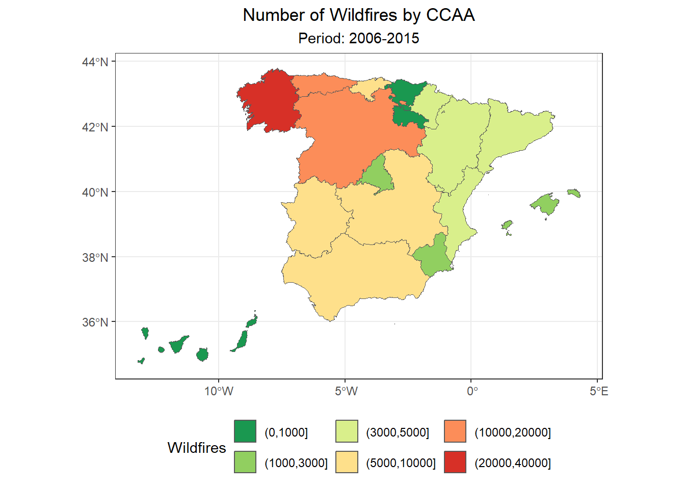
5.1 Analysing the results
We can now confirm that the North-Western area of Spain suffers a significantly higher number of wildfires (>10.000) in comparison to other areas. In contrast, the Eastern area suffers a lesser number of fires, with the Vask Country and La Rioja as the Autonomous Communities which suffered the smallest number of wildfires during the period 2006-2015.